Francoise J.-P., Naber G.L., Tsun T.S. (editors) Encyclopedia of Mathematical Physics
Подождите немного. Документ загружается.


that of the gravity force), M 2R is the total mass of the
body, g 2R is the value of the gravitational accelera-
tion, the fixed point about which the body moves is the
origin, and is the unit vector of the straight line
segment of length ‘ connecting the origin to the center
of mass of the body. This Hamiltonian is left invariant
under rotations about the spatial Oz axis. A momen-
tum map induced by this S
1
-action is given by
J : T
SO(3) !R, J(
h
) = T
e
L
h
(
h
) k;recallthat
T
e
L
h
(
h
) =: 2R
3
is the body angular momentum.
The reduced space J
1
()=S
1
is generically the cotan-
gent bundle of the unit sphere endowed with the
symplectic structure given by the sum of the canonical
form plus a magnetic term; equivalently, this is the
coadjoint orbit in the dual of the Euclidean Lie algebra
se(3)
= R
3
R
3
given by O
= {(, ) j =,
kk
2
= 1}. The projection map J
1
() !O
imple-
menting the symplectic diffeomorphism between the
reduced space and the coadjoint orbit in se(3)
is
given by
h
7!(, ):= (T
e
L
h
(
h
), h
1
k). The orbit
symplectic form !
on O
has the expression
!
(, )(( x þ y, x), ( x
0
þ y
0
,
x
0
)) = (x x
0
) (x y
0
x
0
y) for any
x, x
0
, y, y
0
2R
3
. The heavy-top equations
˙
= þ
Mg‘ ,
˙
= are Lie–Poisson equations on
se(3)
for the Hamiltonian h(, ) = (1=2) þ
Mg‘ and the Lie–Poisson bracket {f , g}(, ) =
(r
f r
g) (r
f r
g r
g r
f ),
where r
and r
denote the partial gradients.
Let ((t), (t)) be a periodic orbit of period T of
the heavy-top equations. After time T, by how much
has the heavy top rotated in space? The answer is
provided by [3]:
’ ¼
1
ZZ
D
!
þ
1
2h
T 2Mg‘
Z
T
0
ðsÞds
¼
ZZ
D
2kIðsÞk
2
ððsÞIðsÞÞðtr IÞ
ððsÞIðsÞÞ
2
ds
þ
Z
T
0
ds
ðsÞIðsÞ
where D is the spherical cap on the unit sphere
whose boundary is the closed curve (t) and D is a
two-dimensional submanifold of the orbit O
bounded by the closed integral curve ((t), (t)).
The first terms in each summand represent the
geometric phase and the second terms the dynamic
phase.
Gauged Poisson Structures
If the Lie group G acts freely and properly on a
smooth manifold Q,then(T
Q)=G is a quotient
Poisson manifold (see Poisson Reduction), where the
quotient is taken relative to the (left) lifted cotangent
action. The leaves of this Poisson manifold are the
orbit reduced spaces J
1
(O
)=G,whereO
g
is
the coadjoint G-orbit through 2g
(see Symmetry
and Symplectic Reduction). Is there an explicit
formula for this reduced Poisson bracket on a
manifold diffeomorphic to (T
Q)=G? It turns out
that this question has two possible answers, once a
connection on the principal bundle : Q !Q=G is
introduced. The discussion below will also link to
the fibration version of cotangent bundle reduction.
In order to present these answers, we review two
bundle constructions. Let G act freely and properly
on the manifold P and consider the a (left) principal
G-bundle : P !P=G := M. Let : N !M be a
surjective submersion. Then the pullback bundle
˜
:(n, p) 2
~
P := {(n, p) 2N P j (p) = (n)} 7!n 2N
over N is also a principal (left) G-bundle relative to
the action g (n, p):= (n, g p).
If there is a (left) G-action a manifold
V, then the
diagonal G-action g (p, v) = (g p, g v)onP V is
also free and proper and one can form the asso-
ciated bundle P
G
V := (P V)=G which is a
locally trivial fiber bundle
E
:[p, v] 2E := P
G
V 7! (p) 2M over M with fibers diffeomorphic to
V. Analogously, one can form the associated fiber
bundle
~
E
:
~
E :=
~
P
G
V !N. Summarizing, the
associated bundle
~
E =
~
P
G
V !N is obtained
from the principal bundle : P !M, the surjective
submersion : N !M, and the G-manifold V by
pullback and association, in this order.
These operations can be reversed. First, form the
associated bundle
E
: E = P
G
V !M and then
pull it back by the surjective submersion : N !M
to N to get the pullback bundle
~
E
:
~
E !N. The map
:
~
P
G
V !
~
E defined by ([(n, p), v]) := (n,[p, v])
is an isomorphism of locally trivial fiber bundles.
These general considerations will be used now to
realize the quotient Poisson manifold (T
Q)=G in
two different ways. Let Q be a manifold and G a Lie
group (with Lie algebra g) acting freely and properly
on it. Let A 2
1
(Q; g ) be a connection 1-form on
the left G-principal bundle : Q !Q=G. Pull back
the G-bundle : Q !Q=G by the cotangent bundle
projection
Q=G
: T
(Q=G) !Q=G to T
(Q=G)to
obtain the G-principal bundle ~
Q=G
:(
[q]
, q) 2
~
Q :=
{(
[q]
, q) j[q] = (q), q 2Q} 7!
[q]
2T
(Q=G). This
bundle is isomorphic to the annihilator (VQ)
T
Q of the vertical bundle VQ := ker T TQ.
Next, form the coadjoint bundle
S
: S :=
~
Q
G
g
!T
(Q=G)of
~
Q,
S
((
[q]
, q), ) =
[q]
, that is,
the associated vector bundle to the G-principal
bundle
~
Q !T
(Q=G) given by the coadjoint repres-
entation of G on g
. The connection-dependent map
A
: S !(T
Q)=G defined by
A
([(
[q]
, q), ]) :=
[T
q
(
[q]
) þ A(q)
], where q 2Q,
q
2T
q
Q, and
Cotangent Bundle Reduction 665

2g
, is a vector bundle isomorphism over Q=G.
The Sternberg space is the Poisson manifold (S,{ , }
S
),
where { , }
S
is the pullback to S by
A
of the quotient
Poisson bracket on (T
Q)=G.
Next, we proceed in the opposite order. Construct
first the coadjoint bundle
~
g
:[q, ] 2
e
g
:= Q
G
g
7![q] 2Q=G associated to the principal bundle
: Q !Q=G and then pull it back by the cotangent
bundle projection
Q=G
: T
(Q=G) !Q=G to
T
(Q=G) to obtain the vector bundle
W
: W :=
{(
[q]
,[q, ]) j
Q=G
(
[q]
) =
~
g
([q, ]) = [q]},
W
(
[q]
,
[q, ]) =
[q]
over T
(Q=G). Note that W = T
(Q=G)
e
g
and hence W is also a vector bundle over
Q/G.LetHQ be the horizontal sub-bundle defined by
the connection A;thus,TQ = HQ VQ,where
H
q
Q := ker A(q). For each q 2Q, the linear map
T
q
j
H
q
Q
: H
q
Q !T
[q]
(Q=G) is an isomorphism. Let
hor
q
:= (T
q
j
H
q
Q
)
1
: T
[q]
(Q=G) !H
q
Q T
q
Q be
the horizontal lift operator induced by the connection
A. Thus, hor
q
: T
q
Q ! T
[q]
(Q=G) is a linear surjective
map whose kernel is the annihilator (H
q
Q)
of the
horizontal space. The connection-dependent map
A
:(T
Q)=G ! W defined by
A
([
q
]) := (hor
q
(
q
), [q, J(
q
)]), where q 2Q,
q
2 T
q
Q,andJ : T
Q !g
is the momentum map of the lifted action,
hJ(
q
), i=
q
((
Q
(q)) for 2g, is a vector bundle
isomorphism over Q/G and
A
A
=.TheWein-
steinspaceisthePoissonmanifold(W,{ , }
W
), where
{ , }
W
is the push-forward by
A
of the Poisson
bracket of (T
Q)=G.Inparticular, : S !W is a
connection independent Poisson diffeomorphism. The
Poisson brackets on S and on W are called gauged
Poisson brackets. They are expressed explicitly in terms
of various covariant derivatives induced on S and on
W by the connection A 2
1
(Q; g ).
Recall that the connection A on the principal
bundle : Q !Q=G naturally induces connections
on pullback bundles and affine connections on
associated vector bundles. Thus, both S and W
carry covariant derivatives induced by A. They are
given, according to general definitions, in the cases
under consideration, by:
If f 2C
1
(S), s = [(
[q]
, q), ] 2S, and v
[q]
2T
[q]
T
(Q=G), then d
S
~
A
f (s) 2T
[q]
T
(Q=G) is defined
by d
S
~
A
f (s)(v
[q]
):= df (s)ðT
((
[q]
, q), )
~
Qg
v
[q]
, hor
q
(T
[q]
(v
[q]
))Þ,0ÞÞ where
~
Qg
:
~
Q g
!
~
Q
G
g
= S is the orbit map. The symbol d
S
~
A
signifies
that this is a covariant derivative on the
associated bundle S induced by the connection
~
A on the principal G-pullback bundle
~
Q !T
(Q=G). This connection
~
A is the pullback
connection defined by A.
If f 2C
1
(W), w = (
[q]
,[q, ]) 2W, and v
[q]
2T
[q]
T
(Q=G), then
e
r
W
A
f (w) 2T
[q]
T
(Q=G) is defined
by
e
r
W
A
f (w)(v
[q]
) = df (w)(v
[q]
, T
(q, )
Qg
(hor
q
(T
[q]
Q=G
(v
[q]
)), 0)) where
Qg
: Q g
!
Q
G
g
=
e
g
is the orbit map. The symbol
e
r
W
A
signifies that this is a covariant derivative on the
pullback bundle W induced by the covariant
derivative r
A
on the coadjoint bundle
e
g
.This
covariant derivative r
A
is induced on
e
g
by the
connection A.
For f 2C
1
(W), we have d
S
~
A
(f ) = (
e
r
W
A
f ) .
To write the two gauged Poisson brackets on S and
on W explicitly, we denote by
~
g = Q
G
g the
adjoint bundle of : Q !Q=G,by
Q=G
the
canonical symplectic structure on T
(Q=G), by
B 2
2
(Q; g ) the curvature of A, and by B the
~
g-valued 2-form B2
2
(Q=G;
~
g) on the base Q=G
defined by B([q])(u
[q]
, v
[q]
) = [q, B(q)(u
q
, v
q
)], for any
u
q
, v
q
2T
q
Q that satisfy T
q
(u
q
) = u
[q]
and
T
q
(v
q
) = v
[q]
. Note that both S
and W
are Lie
algebra bundles, that is, their fibers are Lie algebras
and the fiberwise Lie bracket operation depends
smoothly on the base point. If f 2C
1
(S), denote by
f = s 2S
=
~
Q
G
g the usual fiber derivative of f.
Similarly, if f 2C
1
(W) denote by f =w 2W
the
usual fiber derivative of f. Finally, ] : T
(T
(Q=G)) !T(T
(Q=G)) is the vector bundle iso-
morphism induced by
Q=G
. The Poisson bracket of
f , g 2C
1
(S) is given by
ff ; gg
S
ðsÞ¼
Q=G
ð
½q
Þ d
S
~
A
f ðsÞ
]
; d
S
~
A
gðsÞ
]
s;
f
s
;
g
s
þ v; ð
Q=G
BÞð
½q
Þ d
S
~
A
f ðsÞ
]
; d
S
~
A
gðsÞ
]
DE
where v = [q, ] 2
e
g
. The Poisson bracket f , g 2
C
1
(W) is given by
ff ; gg
W
ðwÞ¼
Q=G
ð
½q
Þ
e
r
W
A
f ðwÞ
]
;
e
r
W
A
gðwÞ
]
w;
f
w
;
g
w
þ v; ð
Q=G
BÞð
½q
Þ
e
r
W
A
f ðwÞ
]
;
e
r
W
A
gðwÞ
]
DE
Note that their structure is of the form: ‘‘canonical’’
bracket plus a (left) ‘‘Lie–Poisson’’ bracket plus a
curvature coupling term.
The Symplectic Leaves of the Sternberg
and Weinstein Spaces
The map ’
A
:
~
Q g
!T
Q given by ’
A
((
[q]
, q),
):= T
q
(
[q]
) þ A(q)
, where ((
[q]
,q),)2
~
Q g
,
is a G-equivariant diffeomorphism; the G-action
on T
Q is by cotangent lift and on
~
Q g
is
g ((
[q]
,q),)=((
[q]
,g q),Ad
g
1
). The pullback J
A
666 Cotangent Bundle Reduction

of the momentum map to
~
Q g
has the expression
J
A
((
[q]
,q),)=,soifOg
is a coadjoint orbit we
have J
1
A
(O)=
~
Q O, and hence the orbit reduced
manifold J
1
A
(O)=G, whose connected components
are the symplectic leaves of S, equals
~
Q
G
O. Its
symplectic form is the Sternberg minimal coupling
form
~
!
O
þ
S
Q=G
.
In this formula, the 2-form
~
!
O
has not been
defined yet. It is uniquely defined by the identity
~
Qg
~
!
O
= d
b
A þ
O
!
O
, where !
O
is the minus orbit
symplectic form on O (see Symmetry and Symplectic
Reduction),
O
:
~
Q O!Ois the projection on the
second factor, and
b
A 2
2
(
~
Q O) is the 2-form
given by
b
A((
[q]
, q), )((u
[q]
, v
q
), ) =
, A(q)(v
q
)
for ((
[q]
, q), ) 2
~
Q O,(u
[q]
, v
q
) 2
T
(
[q]
, q)
~
Q, and 2g
.
The symplectic leaves of the Weinstein space
W are obtained by pushing forward by the
symplectic leaves of the Sternberg space. They are
the connected components of the symplectic
manifolds (T
(Q=G) (Q
G
O),
T
(Q=G)
Q=G
þ
Q
G
O
!
Q
G
O
), where O is a coadjoint orbit in g
,
Q=G
is the canonical symplectic form on T
(Q=G),
!
Q
G
O
is a closed 2-form on Q
G
O to be defined
below, and
T
(Q=G)
: T
(Q=G) (Q
G
O) !
T
(Q=G),
Q
G
O
: T
(Q=G) (Q
G
O) !Q
G
O
are the projections. The closed 2-form !
Q
G
O
2
2
(Q
G
O) is uniquely determined by the identity
Q O
!
Q
G
O
= !
QO
, where
QO
:Q O!Q
G
O
is the orbit space projection, !
QO
2
2
(Q O)is
closed and given by !
QO
(q,)((u
q
, ad
),
(v
q
, ad
)) := d(Aid
O
)(q, )((u
q
, ad
), (v
q
,
ad
)) þ !
O
()(ad
,ad
), and Aid
O
2
1
(Q
g
) is given by (Aid
O
)(q, )(u
q
, ad
) =
, A(q)(u
q
)
,forq 2Q, 2g
, u
q
, v
q
2T
q
Q, , 2g .
Thus, on the Sternberg and Weinstein spaces,
both the Poisson bracket as well as the symplectic
form on the leaves have explicit connection
dependent formulas (see Gauge Theory: Mathema-
tical Applications for a general treatment of gauge
theories).
See also: Gauge Theory: Mathematical Applications;
Hamiltonian Group Actions; Poisson Reduction;
Symmetries and Conservation Laws; Symmetry and
Symplectic Reduction.
Further Reading
Abraham R and Marsden JE (1978) Foundations of Mechanics,
2nd edn. Reading, MA: Addison-Wesley.
Guichardet A (1984) On rotation and vibration motions of
molecules. Annales de l’Institut Henri Poincare´. Physique
The´orique 40: 329–342.
Iwai T (1987) A geometric setting for classical molecular
dynamics. Annales de l’Institut Henri Poincare´. Physique
The´orique. 47: 199–219.
Kummer M (1981) On the construction of the reduced phase
space of a Hamiltonian system with symmetry. Indiana
University Mathematics Journal 30: 281–291.
Lewis D, Marsden JE, Montgomery R, and Ratiu TS (1986) The
Hamiltonian structure for dynamic free boundary problems.
Physica D 18: 391–404.
Marsden JE, Montgomery R, and Ratiu TS (1990) Reduction,
symmetry, and phases in mechanics. Memoirs of the American
Mathematical Society 88(436).
Marsden JE, Misiołek G, Ortega J-P, Perlmutter M, and Ratiu TS
(2005) Hamiltonian Reduction by Stages, Lecture Notes in
Mathematics. Springer.
Marsden JE and Perlmutter M (2000) The orbit bundle picture of
cotangent bundle reduction. Comptes Rendus Mathe´matiques de
l’Acade´mie des Sciences. La Socie´te´ Royale du Canada
22: 33–54.
Marsden JE and Ratiu TS (2003) Introduction to Mechanics and
Symmetry, 2nd edn. second printing; 1st edn. (1994), Texts in
Applied Mathematics, vol. 17. New York: Springer.
Montgomery R (1984) Canonical formulations of a particle in a
Yang–Mills field. Letters in Mathematical Physics 8: 59–67.
Montgomery R (1991) How much does a rigid body rotate? A
Berry’s phase from the eighteenth century. American Journal
of Physics 59: 394–398.
Montgomery R, Marsden JE, and Ratiu TS (1984) Gauged Lie
Poisson structures. In: Marsden J (ed.) Fluids and Plasmas:
Geometry and Dynamics, Contemporary Mathematiques,
vol. 28, pp. 101–114. Providence, RI: American Mathematical
Society.
Satzer WJ (1977) Canonical reduction of mechanical systems
invariant under abelian group actions with an application to
celestial mechanics. Indiana, University Mathematics Journal
26: 951–976.
Simo JC, Lewis D, and Marsden JE (1991) The stability of relative
equilibria. Part I: The reduced energy–momentum method.
Archive for Rational Mechanics and Analysis 115: 15–59.
Smale S (1970) Topology and mechanics. Inventiones Mathema-
ticae 10: 305–331, 11: 45–64.
Sternberg S (1977) Minimal coupling and the symplectic mechanics of
a classical particle in the presence of a Yang–Mills field.
Proceedings of the National Academy of Sciences 74: 5253–5254.
Weinstein A (1978) A universal phase space for particles in Yang–
Mills fields. Letters in Mathematical Physics 2: 417–420.
Zaalani N (1999) Phase space reduction and Poisson structure.
Journal of Mathematical Physics 40(7): 3431–3438.
Cotangent Bundle Reduction 667

Critical Phenomena in Gravitational Collapse
C Gundlach, University of Southampton,
Southampton, UK
ª 2006 Elsevier Ltd. All rights reserved.
Introduction
Sufficiently dense concentrations of mass–energy in
general relativity collapse irreversibly and form black
holes. More precisely, the singularity theorems state
that once a closed trapped surface has developed, some
world lines will only extend to a finite length in the
future – they end in a spacetime singularity. Further-
more, the cosmic censorship hypothesis states that this
singularity is hidden away inside a black hole. One
can, therefore, classify initial data in general relativity
which describe an isolated system with no black hole
present into those which remain regular, and those
which form a black hole during their evolution.
Theorems on the stability of Minkowski spacetime,
and similar results for some types of matter coupled to
gravity, imply that sufficiently weak (in some technical
sense) initial data will remain regular. On the other
hand, no necessary or sufficient criterion for black hole
formation is known. For very strong data the existence
of a closed trapped surface implies black hole
formation, but although the data themselves may be
regular, the trapped surface must already be inside the
black hole. Between the very weak and very strong
regime, there is a middle regime of initial data for
which one cannot decide if they will or will not form a
black hole, other than evolving them in time.
The threshold between collapse and dispersion was
first explored systematically by Choptuik (1992). He
concentrated on the simple model of a spherically
symmetric massless scalar (matter) field (r, t). In this
model, the scalar-field matter must either form a black
hole, or disperse to infinity – it cannot form stable
stars. Choptuik explored the space of initial data by
means of one-parameter families of initial data which
interpolate between strong data (say with large
parameter p) that form a black hole and weak data
(with small p) that disperse. The critical value p
of the
parameter p can be found for each family by evolving
many data sets from that family. Near the black hole
threshold, Choptuik found the following phenomena:
1. Mass scaling. By fine-tuning the initial data to
the threshold along any one-parameter family,
one can make arbitrarily small black holes. Near
the threshold, the black hole m ass scales as
M ’ Cðp p
Þ
for p p
½1
for the black hole mass M in the limit p !p
from above.
2. Universality. While p
and C depend on the
particular one-parameter family of data, the critical
exponent has a universal value, ’ 0.374, for all
one-parameter families of scalar-field data. Further-
more, for a finite time in a finite region of space, the
solutions generated by all near-critical data
approach one and the same solution
, called the
critical solution:
ðr; tÞ’
r
L
;
t t
L
½2
The constants t
and L depend again on the
family of initial data, but
(r, t) is universal. This
universal phase ends when the evolution decides
between black hole formation and dispersion.
The universal critical solution is approached by
any initial data that are sufficiently close to the
black hole threshold, on either side, and from any
one-parameter family.
3. Scale-echoing. The critical solution
(r, t)is
unchanged when one rescales space and time by
afactore
:
ðr; tÞ¼
e
r; e
t
½3
where ’ 3.44 for the scalar field.
The same phenomena were quickly discovered in
many other types of matter coupled to gravity, and
even in vacuum gravity (where gravitational waves can
form black holes). The echoing period and critical
exponent depend on the type of matter, but the
existence of the phenomena appears to be generic. For
some types of matter (e.g., perfect fluid matter), the
critical solution is continuously scale invariant (or
continuously self-similar, CSS) in the sense that
ðr; tÞ¼
ðr=tÞ½4
rather than scale-periodic (or disc retely self-similar,
DSS) as in [3]. (We use the notation
(x) for the
function of one variable r=t.) We have described
scale invariance and scale-echoing here in terms
of coordinates, but these do admit geometric,
coordinate-invariant definitions, which are not
restricted to spherical symmetry.
There is also another kind of critical behavior at the
black hole threshold. Here, too, the evolution goes
through a universal critical solution, but it is static,
rather than scale invariant. As a consequence, the mass
of black holes near the threshold takes a universal
finite value (some fixed fraction of the mass of the
critical solution), instead of showing power-law
668 Critical Phenomena in Gravitational Collapse

scaling. In an analogy with first- and second-order
phase transitions in statistical mechanics, the critical
phenomena with a finite mass at the black hole
threshold are called type I, and the critical phenomena
with power-law scaling of the mass are called type II.
At this point, we characterize the degree of rigor
of the various parts of the theory that is summarized
in this article. Critical phenomena were discovered
in the numerical time evolution of generic asympto-
tically flat initial data. Numerical evolution of many
elements of a specific one-parameter family, and
fine-tuning to the black hole threshold along that
family showed self-similarity and mass scaling near
the threshold. Doing this for a number of randomly
chosen one-parameter families suggests that these
phenomena, and in particular the echoing scale
and mass-scaling exponent , are universal between
initial data within one model (e.g., the spherical
scalar field). Numerical experiments, however, can
only explore a finite-dimensional subspace of the
infinite-dimensional space of initial data (phase
space) of the field theory, and so cannot prove
universality.
We go further by applying the theory of dynami-
cal systems to general relativity. The arguments
summarized in the next section would be difficult to
make rigorou s, as the dynamical system under
consideration is infini te dimensional, but they
suggest a focus on fixed points of the dynamical
system and their linear perturbations. Even though
the dynamical systems motivation is not mathema-
tically rigorous, the linearized analysis itself is a
well-defined problem that can be solved numerically
to essentially arbitrar y precision. This proves uni-
versality on a perturbative level, and provides
numerical values of and . A combination of the
global dynamical systems analysis and perturbative
analysis even predicts further critical exponents for
black hole charge and angular momentum. Finally,
critical phenomena have been discovered in a
number of systems (different types of matter and
symmetry restrictions), and this suggests that they
may be generic for some large class of field theories
(although details such as the numerical values of
and do depend on the system), but there is no
conclusive evidence for this at present.
The Dynamical Systems Picture
When we consider general relativity as an infinite-
dimensional dynamical system, a solution curve is a
spacetime. Points along the curve are Cauchy
surfaces in the spacetime, which can be thought of
as moments of time. An important difference
between general relativity and other field theories
is that the same spacetime can be sliced in many
different ways, none of which is preferred. There-
fore, to turn general relativity into a dynamical
system, one has to fix a slicing (and in practice also
coordinates on each slice). In the example of the
spherically symmetric massless scalar field, using
polar slicing and an area rad ial coordinate r, a point
in phase space can be characterized by the two
functions
Z ¼ ðrÞ; r
@
@t
ðrÞ
½5
In spherical symmetry, there are no degrees of
freedom in the scalar field, and Cauchy data for
the metric can be reconstructed from Z using the
Einstein constraints.
The phase space consists of two halves: initial
data whose time evolution always remains regular,
and data which contain a black hole or form one
during time evolution. The numerical evidence
collected from individual one-parameter families of
data suggests that the black hole threshold that
separates the two is a smooth hypersurface. The
mass-scaling law [1] can, therefore, be restated
without explicit reference to one-parameter families.
Let P be any function on phase space such that data
sets with P > 0 form black holes, and data with P < 0
do not, and which is analytic in a neighborhood of
the black hole threshold P = 0. The black hole mass
as a function on phase space is then given by
M ’ FðPÞ P
½6
for P > 0, where F(P) > 0 is an analytic function.
Consider now the time evolution in this dynami-
cal system, near the threshold (‘‘critical surface’’)
between black hole formation and dispersion. A
phase-space trajectory that starts out in a critical
surface by definition never leaves it. A critical
surface is, therefore, a dynamical system in its own
right, with one dimension fewer. If it has an
attracting fixed point, such a point is called a
critical point. It is an attractor of codimension 1,
and the critical surface is its basin of attraction. The
fact that the critical solution is an attractor of
codimension 1 is visible in its linear perturbations: it
has an infinite number of decaying perturbation
modes tangential to (and spanning) the critical
surface, and a single growing mode not tangential
to the critical surface.
Any trajectory beginning near the critical surface,
but not necessarily near the critical point, moves
almost parallel to the critical surface toward the
critical point. As the phase point approaches the
critical point, its movement parallel to the surface
Critical Phenomena in Gravitational Collapse 669
slows down, while its distance and velocity out of
the critical surface are still small. The phase point
spends sometime moving slowly near the critical
point. Eventually, it moves away from the critical
point in the direction of the growing mode, and ends
up on an attracting fixed point.
This is the origin of universality: any initial data
set that is close to the black hole threshold (on either
side) evolves to a spacetime that approximates the
critical spacetime for sometime. When it fina lly
approaches either the dispersion fixed point or the
black hole fixed point, it does so on a trajectory that
appears to be coming from the critical point itself.
All near-critical solutions are passing through one of
these two funnels. All details of the initial data have
been forgotten, except for the distance from the
black hole threshold: the closer the initial phase
point is to the critical surface, the more the solution
curve approaches the critical point, and the longer it
will remain close to it.
In all systems that have been examined, the black
hole threshold contains at least one critical point. A
fixed point of the dynamical system represents a
spacetime with an additional continuous symmetry
that generic solutions do not have. If the critical
spacetime is time independent in the usual sense, we
have type I critical phenomena; if the symmetry is
scale invariance, we have type II critical phenomena.
The attractor within the critical surface may also be
a limit cycle, rather than a fixed point. In spacetime
terms this corresponds to a discrete symmetry (DSS
rather than CSS in type II, or a pulsating critical
solution, rather than a stationary one , in type I).
Self-Similarity and Mass Scaling
Type II critical phenomena occur where the critical
solution is scale invariant (self-similar, CSS or DSS).
Using suitable spacetime coordinates, a CSS solution
can be characterized as independent of a time
coordinate which is also a logarithmic scale.
Similarly, a DSS solution can be characterized as
periodic in . For example, starting from the scale
periodicity [3] in polar-radial coordinates, we
replace r and t by new coordinates
x
r
t t
;ln
t t
L
½7
where the accumulation time t
and scale L must be
matched to the one-parameter family under con-
sideration. has been defined so that it increases as
t increases and approaches t
from below. It is useful
to think of r, t, and L as having dimension length in
units c = G = 1, and of x and as dimensionless.
Choptuik’s observation, expressed in these coordi-
nates, is that in any near-critical solution there is
a spacetime region where the fields Z are well
approximated by the critical solution, or
Zðx;Þ’Z
ðx;Þ½8
with
Z
ðx;þÞ¼Z
ðx;Þ½9
Note that the time parameter of the dynamical
system must be chosen as if a CSS solution is to be
a fixed point, or a DSS solution a cycle. More
generally (going beyond spherical symmetry), on any
self-similar spacetime one can intro duce coordinates
x
= (, x
1
, x
2
, x
3
) in which the metric is of the form
g
¼ e
2
g
½10
and where
¯
g
is independent of for a CSS
spacetime, and periodic in for a DSS spacetime.
These coordinates are not unique.
The critical exponent can be calculated from the
linear perturbations of the critical solution. In order
to keep the notation simple, the discussion will be
restricted to a critical solution that is spherically
symmetric and CSS, whi ch is correct, for example,
for perfect-fluid matter.
Let us assume that we have fine-tuned initial data
close to the black hole threshold so that in a region
the resulting spacetime is well approximated by the
CSS critical solution. This part of the spacetime
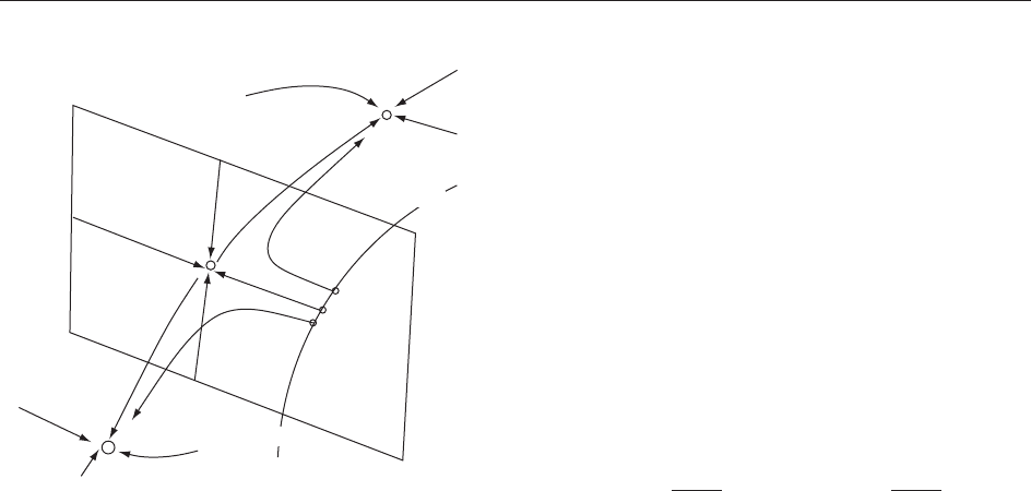
Black hole
threshold
Critical
point
Flat space fixed point
p
< p
*
p
= p
*
p
> p
*
Black hole fixed point
One-paramete
r
family of
initial data
Figure 1 The phase-space picture for the black hole threshold
in the presence of a critical point. The arrow lines are time
evolutions, corresponding to spacetimes. The line without an
arrow is not a time evolution, but a one-parameter family of initial
data that crosses the black hole threshold at p = p
. (Reproduced
with permission from Gundlach C (2003) Critical phenomena in
gravitational collapse. Physics Reports 376: 339–405.)
670 Critical Phenomena in Gravitational Collapse

corresponds to the section of the phase-space
trajectory that lingers near the critical point. In this
region, we can linearize around Z
.AsZ
does not
depend on , its linear perturbations can depend
on only exponentially. Labeling the perturbation
modes by i, a single mode perturb ation is of
the form
Z ¼ C
i
e
i
Z
i
ðxÞ½11
In the near-critical regime, we can therefore
approximate the solution as
Zðx;Þ’Z
ðxÞþ
X
1
i¼0
C
i
ðpÞe
i
Z
i
ðxÞ½12
The notation C
i
(p) is used because the perturbation
amplitudes C
i
depend on the initial data, and hence
on the parameter p that controls the initial data.
If Z
is a critical solution, by definition there is
exactly one
i
with positive real part (in fact, it is
purely real), say
0
.Ast !t
from below, which
corresponds to !1, all other perturbations decay
and can be neglected. By definition, the critical
solution corresponds to p = p
, and so we must have
C
0
(p
) = 0. Linearizing around p
, we obtain
Zðx;Þ’Z
ðxÞþ
dC
0
dp
p
ðp p
Þe
0
Z
0
ðxÞ½13
in a region of the spacetime.
Now we extract Cauchy data at one particular
value of within that region, namely at
p
defined by
dC
0
dp
p
jp p
je
0
p
½14
where is an arbitrary small constant, so that
Zðx;
p
Þ’Z
ðxÞ Z
0
ðxÞ½15
where is the sign of p p
, left behind because by
definition is positive. As increases from
p
, the
growing perturbation becomes nonlin ear and the
approximation [13] breaks down. Then either a
black hole forms (say for the positive sign), or the
solution disperses (for the negative sign). We need
not follow this nonlinear evolution in detai l to find
the black hole mass scaling in the former case:
dimensional analysis is sufficient. Going back to
coordinates t and r, we have
Zðr; t
p
Þ’Z
r
L
p
Z
0
r
L
p
½16
where
L
p
Le
p
½17
These Cauchy data at t = t
p
depend on the initial
data at t = 0 only through the overall scale L
p
, and
through the sign in front of . If the field equations
themselves are scale invariant, or asymptotically
scale invariant at scales L
p
and smaller, the black
hole mass, which has dimensions of length in
gravitational units, must be proportional to the
initial data scale L
p
, the only length scale that is
present. Therefore,
M / L
p
/ðp p
Þ
1=
0
½18
and we have found the critical exponent to be = 1=
0
.
The Analogy with Statistical Mechanics
The existence of a threshold where a qualitative
change takes place, universality, scale invariance,
and critical exponents suggest that there i s a
mathematical analogy between type II critical
phenomena and c ritical phase transitions in statis-
tical mechanics.
In equilibrium statistical mechanics, observable
macroscopic quantities, such as the magnetization of
a ferromagnetic material, are derived as statistical
averages over microstates of the system. The
expected value of an observable is
hAi¼
X
microstates
AðmicrostateÞ e
Hð microstate;Þ
½19
The Hamiltonian H depends on the parameters ,
which comprise the temperature, parameters char-
acterizing the system such as interaction energies of
the constitue nt molecules, and macroscopic forces
such as the external magnetic field. The objective of
statistical mechanics is to derive relations between
the macroscopic quantities A and parameters .
Phase transitions in thermodynamics are thresholds
in the space of external forces at which the
macroscopic observables A, or one of their derivatives,
change discontinuously. In a ferromagnetic material
at high temperatures, the magnetization m of the
material (alignment of atomic spins) is determined by
the external magnetic field B. At low temperatures, the
material shows a spontaneous magnetization even at
zero external field, which breaks rotational symmetry.
With increasing temperature, the spontaneous magne-
tization m decreases and vanishes at the Curie
temperature T
as
jmjðT
TÞ
½20
In the presence of a very weak external field, the
spontaneous magnetization aligns itself with the
external field B, while its strength is, to leading
order, independent of B. The function m(B, T),
Critical Phenomena in Gravitational Collapse 671

therefore, changes discontinuously at B = 0. The line
B = 0 for T < T
is, therefore, a line of first-order
phase transitions between the possible directions of
the spontaneous magnetization (in a one-dimen-
sional system, between m up and m down). This line
ends at the critical point (B = 0, T = T
) where the
order parameter jmj vanishes. The role of B = 0as
the critical value of B is obscured by the fact that
B = 0 is singled out by symmetry.
A critical phase transition involves scale-invariant
physics. One sign of this is that fluctuations appear
on a large range of length scales between the
underlying atomic scale and the scale of the sampl e.
In particular, the atomic scale, and any dimensionful
parameters associated with that scale, must become
irrelevant at the critical point. This can be taken as
the starting point for obtaining properties of the
system at the critical point.
One first defines a semigroup acting on micro-
states: the renormalization group. Its action is to
group together a small number of particles as a
single particle of a fictitious new system, using some
averaging procedure. Alternatively, this can also be
done in Fourier space. One then defines a dual
action of the renormalization group on the space of
Hamiltonians by demanding that the partition
function is invariant under the renormalization
group action:
X
microstates
e
H
¼
X
microstates
0
e
H
0
½21
The renormalized Hamiltonian H
0
is in general
more complicated than the original one, but it can
be approximated by a f ixed expression where only
a finite number of parameters are adjusted. Fixed
points of the renormalization group correspond to
Hamiltonians w ith the parameters at their critical
values. The critical value of any dimensional
parameter must be zero (or infinity). Only
dimensionless combinations can have nontrivial
critical values.
The behavior of thermodynamical quantities at
the critical point is in general not trivial to calculate.
But the action of the renormalization group on
length scales is given by its definition. The blowup
of the correlation length at the critical point is,
therefore, the easiest critical exponent to calculate.
We make contact with critical phenomena in
gravitational collapse by considering the time evolu-
tion in coordinates (, x) as a renormalization group
action. The calculation of the critical exponent for
the black hole mass M is the precise an alog of the
calculation of the critical exponent for the correla-
tion length , substituting T
T for p p
, and
taking into account that the -evolution in critical
collapse is toward smaller scales, while the renor-
malization group flow goes toward larger scales:
therefore, diverges at the cri tical point, while M
vanishes.
We have shown above that the black hole mass is
controlled by one global function P on phase space.
Clearly, P is the gravity equivalent of T T
in
the ferromagnet. But it is tempting to speculate
(Gundlach 2002)that there is also a gravity equiva-
lent of the external magnetic field B, which gives rise
to a second independent critical exponent. At least
in some situations, the angular momentum of the
initial data can play this role. Note that, like B,
angular momentum is a vector, with a critical value
that is zero because all other values break rotational
symmetry. Furthermore, the final black hole can
have nonvanishing angular momentum, which must
depend on the angular momentum of the initial
data. The former is analogous to the magnetization
m, the latter to the external field B. It can be shown
that this analogy holds perturbatively for small
angular momentum. Future numerical simulations
will show if it goes further.
Universality and Cosmic Censorship
Critical phenomena in gravitational collapse first
generated interest because a complicated self-similar
structure and dimensionless numbers and arise
from generic initial data evolved by quite simple
field equations. Another point of interest is the
rather detai led analogy of phenomena in a determi-
nistic field theory with critical phase transitions in
statistical mechanics. But critical phenomena are
important for general relativity mostly for a differ-
ent reason.
Black holes are among the most important
solutions of general relativity because of their
universality: the black hole uniqueness theorems
state that stable black holes are completely deter-
mined by their mass, angular momentum, and
electric charge – the Kerr–Newman family of black
holes. Perturbation theory shows that any perturba-
tions of black holes from the Kerr–Newman solu-
tions must be radiated away.
Critical soluti ons have a similar importance
because they are generic intermediate states of
the evolution that are also independent of the
initial data. An important distinction is that
critical solutions depend on the m atter model,
and are therefore less universal than black holes.
However, critical phenomena in gravitational
collapse s eem to arise in axisymmetric vacuum
spacetimes, and so are apparently not linked to the
672 Critical Phenomena in Gravitational Collapse

presence of matter. Furthermore, they also a rise in
perfect-fluid matter w ith the equation of state
p = =3, which is that of an ultrarelativisti c gas.
This is a good approximation for matter at very
high density, such as in the big bang. This is
important because critical phenomena probe
arbitraril y large matter densities or spacetime
curvatures as the initial data are fine-tuned to the
black hole threshold. At even higher densities,
presumably on the Planck scale, s cale invariance is
again broken by quantum-gravity effects, and
so critical phenomena will end there.
The cosmic censorship conjecture states that
naked singularities do not arise from suitably
generic initial data for suitably well-behaved mat-
ter. Critical phenomena in gravitational collapse
have forced a tightening of this conjecture. Type II
(self-similar) critical solutions contain a naked
singularity, that is, a point of infinite spacetime
curvature from which information can reach a
distant observer. (By contrast, the singularity inside
a black hole is hidden from distant observers.) On a
kinematical level, this could be seen already from
the form [10] of the metric. Because the critical
solution is the end state for all initial data that are
exactly on the black hole threshold, all initial data
on the black hole threshold form a naked singular-
ity. As type II critical phenomena appear to be
generic at least in spherical symmetry, this means
that in generic self-gravitating systems, the space of
regular initial data that form naked singularities is
larger than expected, namely of codimension 1.
Excluding naked singularities from generic initial
data may be the sharpest version of cosmic censor-
ship one can now hope to prove.
Another point of interest in critical collapse is that
it allows one to make a small region of arbitrarily
high curvature from finite-curvature initial data.
This may be a route for probing quantum-gravity
effects. Similarly, one can make black holes that are
much smaller than any length scale present in the
initial data or the matter equation of state. An
application has been suggested for this in cosmol-
ogy, where primordial black holes could have
masses much smaller than the Hubble scale at
which they are created, rather than of the order of
this scale.
Outlook
Critical phenomena in gravitational collapse are now
well understood in spherical symmetry, both theoreti-
cally and in numerical simulations. In some matter
models, the phenomenology is quite complicated, but
it still fits into the basic picture outlined here.
The crucial question as to what happens beyond
spherical symmetry remains largely unanswered at
the time of writing. Perturbation theory around
spherical symmetry suggests that c ritical phenom-
ena are not restricted to exactly spherical situa-
tions. This is also s upported by simulations in
axisymmetric (highly nonspherical) vacuum grav-
ity. Other simulations of nonspherical gravitational
collapse which cover the necessary range of space-
timescalesrequiredtosee critical phenomena are
only just becoming available, and the results are
not yet clear-cut. For collapse with angular
momentum, no high-resolution calculations have
yet been carried out. As the necessary techniques
become available, one should be prepared for
numerical simulations to make dramatic extensions
or corrections to the picture of critical collapse
drawn up here.
See also: Computational Methods in General Relativity:
The Theory; Spacetime Topology, Causal Structure and
Singularities; Stability of Minkowski Space; Stationary
Black Holes.
Further Reading
Abrahams AM and Evans CR (1993) Critical behavior and
scaling in vacuum axisymmetric gravitational collapse. Physi-
cal Review Letters 70: 2980–2983.
Choptuik MW (1993) Universality and scaling in gravitational
collapse of a massless scalar field. Physical Review Letters
70: 9–12.
Choptuik MW (1999) Critical behavior in gravitational collapse.
Progress of Theoretical Physics 136 (suppl.): 353–365.
Evans CR and Coleman JS (1994) Critical phenomena and self-
similarity in the gravitational collapse of radiation fluid.
Physical Review Letters 72: 1782–1785.
Gundlach C ( 1999) Living Reviews in Relativity 2: 4 (published
electronically at http://www.livingreviews.org).
Gundlach C (2002) Critical gravitational collapse with angular
momentum: from critical exponents to universal scaling
functions. Physical Review D 65: 064019.
Critical Phenomena in Gravitational Collapse 673

Current Algebra
G A Goldin, Rutgers University, Piscataway, NJ, USA
ª 2006 Elsevier Ltd. All rights reserved.
Introduction
Certain commutation relations among the current
density operators in quantum field theories define
an infinite-dimensional Lie algebra. The original
current algebra of Gell-Mann described weak and
electromagnetic currents of the strongly interacting
particles (hadrons), leadin g to the Adler–Weisberger
formula and other important physical results. This
helped inspire math ematical and quantum-theoretic
developments such as the Sugawara model, light
cone currents, Virasoro algebra, the mathematical
theory of affine Kac–Moody algebras, and non-
relativistic current algebra in quantum and statis-
tical physics. Lie algebras of local currents may be
the infinitesimal representations of loop groups,
local current groups or gauge groups, diffeomorph-
ism groups, and their semidirect products or other
extensions. Broadly construed, current algebra thus
leads directly into the representation theory of
infinite-dimensional groups and algebras. Applica-
tions have ranged across conformally invariant
field theory, vertex operator algebras, exactly
solvable lattice and continuum models in statistical
physics, exotic particle statistics and q-commuta-
tion rel ations, hydrodynamics and quantized vortex
motion. This brief survey describes but a few
highlights.
Relativistic Local Current Algebra
for Hadrons
To model superfluidity, Landau had proposed in
1941 a quantum hydrodynamics fundamentally
based on local fluid densities and currents as
(operator) dynamical variables. However, current
algebra came into its own in theoretical physics with
the ideas of Gell-Mann in the earl y 1960s. The basic
concept, in the era just preceding quantum chromo-
dynamics (QCD), was that even without knowing
the Lagrangian governing hadron dynamics in
detail, exact kinematical information – the local
symmetry – could still be encoded in an algebra of
currents. The local (vector and axial vector) current
density operators, expressed where possible in terms
of underlying quantized field operators in Hilbert
space, were to form two octets of Lorentz 4-vectors,
with each octet corresponding to the eight genera-
tors of the compact Lie group SU(3).
More specifically (Adler and Dashen 1968), let
F
a
(x), a = 1, 2, ...,8, = 0, 1, 2, 3, be an octet of
hadronic vector currents, where as usual
x = (x
) = (x
0
, x) denotes a point in four-dimensional
spacetime. Likewise, introduce an axial vector octet
F
5
a
(x). Unless otherwise specified, we use natural
units, where h = 1 and c = 1. Define the correspond-
ing charges F
a
and F
5
a
to be the space integrals of the
time components of these curre nts, that is,
F
a
ðx
0
Þ¼
Z
d
3
xF
0
a
ðx
0
; xÞ
F
5
a
ðx
0
Þ¼
Z
d
3
xF
50
a
ðx
0
; xÞ
½1
where d
3
x = dx
1
dx
2
dx
3
. Then F
1
, F
2
, F
3
are the
three components I
1
, I
2
, I
3
of the isotopic spin, and
Y = (2
ffiffiffi
3
p
=3)F
8
is the hypercharge. The usual elec-
tromagnetic current J
em
(x
0
, x) is given by
J
em
¼ q F
3
þ
ffiffiffi
3
p
3
F
8
!
½2
where q is the unit elementary charge, and the total
charge is given by Q =
R
d
3
xJ
0
em
(x
0
, x) = q(I
3
þ Y=2).
The hadronic part of the weak current entering an
effective Lagrangian can be written as
J
w
¼F
1
F
5
1
þ i F
2
F
5
2
hi
cos
C
þF
4
F
5
4
þ i F
5
F
5
5
hi
sin
C
½3
where
C
is the Cabibbo angle (determined experi-
mentally to be 0.27 rad). The terms with F
1
F
5
1
and F
2
F
5
2
are strangeness conserving, those with
F
4
F
5
4
and F
5
F
5
5
are not.
The main current algebra hypothesis is that the
time components F
0
and F
50
of these octets satisfy
the equal-time commutation relations:
F
0
a
ðx
0
; xÞ; F
0
b
ðy
0
; yÞ
x
0
¼y
0
¼ i
ð3Þ
ðx yÞ
X
d
c
abd
F
0
d
ðx
0
; xÞ
F
0
a
ðx
0
; xÞ; F
50
b
ðy
0
; yÞ
x
0
¼y
0
¼ i
ð3Þ
ðx yÞ
X
d
c
abd
F
50
d
ðx
0
; xÞ
F
50
a
ðx
0
; xÞ; F
50
b
ðy
0
; yÞ
x
0
¼y
0
¼ i
ð3Þ
ðx yÞ
X
d
c
abd
F
0
d
ðx
0
; xÞ
½4
where the c
abd
are structure constants of the Lie
algebra of SU(3), antisymmetric in the indices. Since
current commutators relate bilinear expressions to
674 Current Algebra