Francoise J.-P., Naber G.L., Tsun T.S. (editors) Encyclopedia of Mathematical Physics

Подождите немного. Документ загружается.

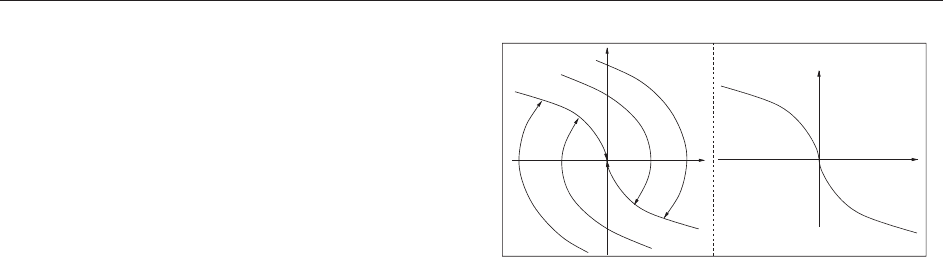
admits a proper strictly plurisubharmonic function

 : X ! R. An important result says that X is Stein

if and only if it can be realized as a closed complex

submanifold of C

. Clearly any noncritical level set

of  gives a contact manifold.

Contact manifolds also give rise to an interesting

class of differential operators. Specifical ly, a contact

structure  on M defines a symbol-filtered algebra of

pseudodifferential operators 





(M), called the

‘‘Heisenberg calculus.’’ Operators in this algebra

are modeled on smooth families of convolution

operators on the Heisenberg group. An important

class of operators of this type are the ‘‘sum-of-

squares’’ operators. Locally, the highest-order part

of such an operator takes the form

L ¼

j¼1

þ iav



½7

where {v

, ..., v

} is a local framing for the contact

field and v



is a Reeb vector field. This operator

belongs to 



(M) and is subel liptic for a outside a

discrete set.

Hamiltonian Dynamics

Given a symplectic manifold (X, !), a function

H : X !R will be called a Hamiltonian. (Only

autonomous Hamiltonians are discussed here.) The

unique vector field satisfying



! ¼dH

is called the Hamiltonian vector field associated to

H. Many problems in classical mechanics can be

formulated in terms of studying the flow of v

for

various H.

Example 8 If (X, !) = (R

,d), where  is from

Example 2, then the flow of the Ham iltonian vector

field is given by

q ¼

;

p ¼

A standard fact says that the flow of v

preserves

the level sets of H.

Theorem 7 If M is a level set of H corresponding

to a regular value and M is a hypersurface of contact

type, then the trajectories of v

and of the Reeb

vector field (associated to M in Theorem 3) agree.

Thus under suitable hypothesis, Hamiltonian

dynamics is a reparametrization of Reeb dynamics.

In particular, searching for periodic orbits in such a

Hamiltonian system is equivalent to searching for

periodic orbits in a Reeb flow. Thus in this context,

Weinstein’s conjecture asserts a positive answer to

the questions: Does the Hamiltonian flow along a

regular level set of contact type have a periodic

orbit? Viterbo proved that the answer was yes if the

hypersurface is compact and in (R

, ! = d). Other

progress has been made by studying Reeb dynamics.

Geometric Optics

In this section, we study the propagation of light (or

various other disturbances) in a medium (for the

moment, we do not specify the properties of this

medium). The medium will be given by a three-

dimensional manifold M. Given a point p in M and

t > 0, let I

(t) be the set of all points to whi ch light

can travel in time t. The wave front of p at time t

is the boundary of this set and is denoted as



(t) = @I

(t).

Theorem 8 (Huygens’ principle). 

(t þ t

) is the

envelope of the wave fronts 

) for all q 2 

(t).

This is best understood in terms of contact

geometry. Let  :(T



Mn{0}) !P



M be the natural

projection (see Example 3) and let S be any smooth

sub-bundle of T



Mn{0} that is transverse to the radial

vector field in each fiber and for which  j

: S !P



is a diffeomorphism. The restriction of the Liouville

form to S gives a contact form  and a corresponding

Reeb vector field v. Given a subset F of M with a well-

defined tangent space at every point set

¼fp 2 S : ðpÞ2F and pðwÞ¼0 for all

w 2 T

ðpÞ

Fg½8

The set L

is a Legendrian submanifold of S and is

called the ‘ ‘Legendrian lift’’ of F.IfL is a generic

Legendrian submanifold in S,then(L) is called the

front projection of L and L

(L)

= L. Given a Legendrian

submanifold L,let

(L) be the Legendrian submani-

fold obtained from L by flowing along v for time t.

Example 9 Given a metric g on M, Fermat’s

principle says that light travels along geodesics.

Thus, if S is the unit cotangent bundle, then using g

to identify the geodesic flow with the Reeb flow

one sees that light will travel along trajectories

of the Reeb vector field. Given a point p in M,

the Legendrian submanifold L

is a sphere sitting

in T



M. The Huygens principle follow s from the

observation that 

(t) = (

)).

Using the more general S discussed above, one can

generalize this example to light traveling in a medium

that is nonhomogeneous (i.e., the speed differs from

point to point in M) and anisotropic (i.e., the speed

differs depending on the direction of travel).

Contact Manifolds 635

See also: Hamiltonian Fluid Dynamics; Integrable Systems

and Recursion Operators on Symplectic and Jacobi

Manifolds; Minimax Principle in the Calculus of Variations.

Further Reading

Aebisher B, Borer M, Ka¨lin M, Leuenberger Ch, and Reimann

HM (1994) Symplectic Geometry, Progress in Mathematics,

vol. 124. Basel: Birkha¨ user.

Arnol’d VI (1989) Mathematical Methods of Classical Mechanics,

Graduate Texts in Mathematics, vol. 60, xviþ516, pp. 163–179.

New York: Springer.

Arnol’d VI (1990) Contact Geometry: The Geometrical Method of

Gibbs’s Thermodynamics, Proceedings of the Gibbs Symposium.

(New Haven, CT, 1989), pp. 163–179. Providence, RI: American

Mathematical Society.

Beals R and Greiner P (1988) Calculus on Heisenberg manifolds.

Annals of Mathematics Studies 119.

Eliashberg Y, Givental A, and Hofer H (2000) Introduction to

Symplectic Field Theory, GAFA 2000 (Tel Aviv, 1999), Geom.

Funct. Anal. 2000, Special Volume, Part II, pp. 560–673.

Etnyre J. Legendrian and transversal knots. Handbook of Knot

Theory (in press).

Etnyre J (1998) Symplectic Convexity in Low-Dimensional

Topology, Symplectic, Contact and Low-Dimensional Topol-

ogy (Athens, GA, 1996), Topology Appl., vol. 88, No. 1–2,

pp. 3–25.

Etnyre J and Ng L (2003) Problems in Low Dimensional Contact

Topology, Topology and Geometry of Manifolds (Athens,

GA, 2001), pp. 337–357, Proc. Sympos. Pure Math., vol. 71.

Providence, RI: American Mathematical Society.

Geiges H Contact geometry. Handbook of Differential Geometry,

vol. 2 (in press).

Geiges H (2001a) Contact Topology in Dimension Greater than

Three, European Congress of Mathematics, vol. II (Barcelona,

2000), Progress in Mathematics, vol. 202, pp. 535–545. Basel:

Birkha¨user.

Geiges H (2001b) A brief history of contact geometry and

topology. Expositiones Mathematicae 19(1): 25–53.

Ghrist R and Komendarczyk R (2001) Topological features of

inviscid flows. An Introduction to the Geometry and Topology

of Fluid Flows (Cambridge, 2000), 183–201, NATO Sci. Ser. II

Math. Phys. Chem., vol. 47. Dordrecht: Kluwer Academic.

Giroux E (2002) Ge´ome´trie de contact: de la dimension trois

vers les dimensions supe´rieures, Proceedings of the Inter-

national Congress of Mathematicians, vol. II (Beijing, 2002),

pp. 405–414. Beijing: Higher Ed. Press.

Hofer H and Zehnder E (1994) Symplectic Invariants and

Hamiltonian Dynamics, Birkha¨user Advanced Texts: Basler

Lehrbu¨ cher, pp. xivþ341. Basel: Birkha¨user.

Taylor ME (1984) Noncommutative Microlocal Analysis, Part I,

Mem Amer. Math. Soc., 52, no. 313. American Mathematical

Society.

Control Problems in Mathematical Physics

B Piccoli, Istituto per le Applicazioni del Calcolo,

Rome, Italy

Introduction

Control Theory is an interdisciplinary research area,

bridging mathematics and engineering, dealing with

physical systems which can be ‘‘controlled,’’ that is,

whose evolution can be influenced by some external

agent. A general model can be written as

yðtÞ¼Að t; yð0Þ; uðÞÞ ½1

where y describes the state variables, y(0) the initial

condition, and u() the control function. Thus, eqn

[1] means that the state at time t depends on the

initial condit ion but also on some parameters u

which can be chosen as function of time. To be

precise, there are some control problems which are

not of evolutiona ry type; however, in this presenta-

tion we restrict ourselves to this case.

One has to distinguish among the control set U where

the control function can take values: u(t) 2U,andthe

space of control functions, U, to which each control

function should belong: u() 2U. Thus, for example,

we may have U = R

and U = L

([0, T], R

There are various problems one can formulate

regarding systems of type [1], among which:

Controllability Given any two states y

and y

determine a control function u() such that for

some time t > 0wehavey

= A(t, y

, u()).

Optimal control Consider a cost function J(y(),

u()) depending both on the evolutions of y and u

and determine a control function

u() and a

trajectory

y(t) = A(t , y

u()) such that

y() steers

the system from y

to y

, as before, and the cost J

is minimized (or maximized).

Stabilization We say that



y is an equilibrium if

there exists



u 2 U such that A(t,



u) =



y for every

t > 0 (here



u indicates also the constant in time

control function). Determine the control u as

function of the state y so that



y is a (Lyapunov)

stable equilibrium for the uncontrolled dynamical

system y(t ) = A(t, y(0), u(y())).

Observability Assume that we can observe not the

state y, but a function (y) of the state. Determine

conditions on  so that the state y can be

reconstructed from the evolution of (y) choosing

u() suitably.

For the sake of simplicity, we restrict ourselves

mainly to the first two problems and just mention

636 Control Problems in Mathematical Physics

some facts about the others. Also, we focus on two

cases:

Control of ordinary differential equations (ODEs)In

this case t 2 R, y 2 R

, U is a set, typically

U  R

,andA is determined by a controlled ODE

y ¼ f ðt; y; uÞ½2

A typical example in mathematical physics is the

control of mechanical systems (Bloch 2003, Bullo

and Lewis 2005).

Control of partial differential equations (PDEs)In

this case t 2 R, x 2 R

, y(x) belongs to a Banach

functional space, for example, H

nþ1

, R), U is a

functional space, and A is determined by a

controlled PDE,

Fðt; x; y; y

; y

; ...; y

; y

; ...; uÞ¼0 ½3

A typical example in mathematical physics is the

control of wave equation using boundary condi-

tions, see below.

There are various other possible situations we do

not treat here: ‘ ‘stochastic control,’ ’ when y is a random

variable and A defined by a (controlled) sto-

chastic differential equation; ‘ ‘discrete time control,’’

where t 2 N; ‘ ‘hybrid control,’ ’ where t and y may have

both discrete and continuous components, and so on.

As shown above, the control law can be assigned

in (at least) two basically different ways. In open-

loop form, as a function of time: t ! u(t), and in

closed-loop form or feedback, as a function of the

state: y ! u(y). For example, in optimal control we

look for a control

u(t) in open-loop form, while in

stabilization we search for a feedback control u(y).

The open -loop control depends on y(0), while a

feedback control can stabilize regardless of the

initial condition.

Example 1 A point with unit mass moves along a

straight line; if a controller is able to apply an

external force u, then, calling y

(t), y

(t), respec-

tively, the position and the velocity of the point at

time t, the motion is described by the control system

;

Þ¼ðy

; uÞ½4

It is easy to check that the feedback control

u(y

, y

) = y

 y

stabilizes the system asymptot-

ically to the origin, that is, for every initial data

(



), the solution of the corresponding Cauchy

problem satisfies lim

t !1

, y

)(t ) = (0, 0).

Another simple problem consists in driving the

point to the origin with zero velocity in minimum

time from given initial data. It is quite easy to see

that the optimal strategy is to accelerate towards the

origin with maximum force on some interval [0, t]

and then to decelerate with maximum force to reach

the origin at velocity zero. The set of optimal

trajectories is depicted in Figure 1a: they can

be obtained using the following discontinuous

feedback, see Figure 1b. Define the curves





= {(y

, y

): y

> 0, y

= y

} and let  be

defined as the union 



[ {0}. We define A

to be

the region below  and A



the one above. Then the

feedback is given by

uðxÞ¼

þ1ifðy

; y

Þ2A

[ 

1ifðy

; y

Þ2A



[ 



0ifðy

; y

Þ¼ð0; 0Þ

Example 2 Consider a (one-dimensional) vibrating

string of unitary length with a fixed endpoint. The

model for the motion of the displacement of the

string with respect to the rest position is given by

þ y ¼ 0; yðt; 0Þ¼0 ½5

with initial data

yð0; Þ ¼ y

; y

ð0; Þ ¼ y

½6

Assume that we can control the position of the

second endpoint; then,

yðt; 1Þ¼uðtÞ½7

for some control function u() 2R.

Let us introduce another key concept: the reach-

able set at time t from



y is the set

Rðt;



yÞ¼fAðt;



y; uðÞÞ: uðÞ2Ug

Various problems can be formulated in terms of

reachable sets, for example, controllability requires

that for every



y the union of all R(t;



y)ast !1

includes the entire space. The dependence of R(t;



on time t and on the set of controls U is also a

subject of investigation: one may ask whether the

same points in R(t;



y) can be reached by using

controls which are piecewise constant, or take

values within some subsets of U.

u(y) = –1

u(y)

= +1

–

+1)

Figure 1 Example 1. The simplest example of (a) optimal

synthesis and (b) corresponding feedback.

Control Problems in Mathematical Physics 637

Control of ODEs

For most proofs we refer to Agrachev and Sachkov

(2004) and Sontag (1998).

Controllability

Consider first the case of a linear system:

y ¼ Ay þ Bu; u 2 U; yð0 Þ¼y

½8

where y, y

2 R

, U  R

, A is an n  n matrix and

B an n  m matrix. We have the following property

of reachable sets:

Theorem 1 If U is compact convex then the

reachable set R(t) for [8] is compact and convex.

A control system [8] is controllable if taking

U = R

we have R(t) = R

for every t > 0. By

linearity, this is equivalent to requiring the reachable

set to be a neighborhood of the origin in case of

bounded controls. Define the controllability matrix

to be the n  nm matrix

CðA; BÞ¼ðB; AB; ...; A

n1

BÞ

Controllability is characterized by the following:

Theorem 2 (Kalman controllability theorem). The

linear system [8] is controllable if and only if

rank(C(A, B)) = n.

For linear systems, there exists a duality between

controllability and observability in the sense of the

following theorem:

Theorem 3 Consider the linear control system [8]

and assume to observe the variable z(y) = Cy for

some p  n matrix C. Then, observability holds if

and only if the linear system

y = A

y þ C

vis

controllable.

There exists no characterization of controllability

for nonlinear systems as for lin ear ones, but we have

the linearization result:

Theorem 4 A nonlinear system is locally control-

lable if its linearization is. The converse is false.

There are many results for the important class of

control–affine systems

y ¼ f

ðyÞþ

i¼1

ðyÞu

½9

where f

, ..., f

are smooth vector fields on R

and

U = R

. In general, there exists no explicit represen-

tation for the trajectories of [9], in terms of integrals

of the control as it happens for linear systems. Still, a

rich mathematical theory has been developed apply-

ing techniques and ideas from differential geometry:

the so-called geometric control theory. The main idea

is that controllability (and properties of optimal

trajectories) is determined by the Lie algebra gener-

ated by vector fields f

. For example:

Theorem 5 (Lie-algebraic rank condition). Let L

be the Lie algebra generated by the vector fields

, i = 1, ..., m, and assume f

= 0. If L(y) is of

dimension n at every point y then the system is

controllable.

We refer to Agrachev and Sachkov (2004)

and Jurdjevic (1997) for general presentation of

geometric control theory and give a simple example

to show how Lie brackets characterize reachable

directions.

Example 3 Consider the Brockett integrator

¼ u

;

¼ u

;

¼ u

 u

Starting from the origin, using constant controls, we

can move along curves tangent to the y

plane.

However, let f

= (1, 0, y

) and f

= (0, 1, y

) (fields

corresponding to constant controls); then their Lie

bracket is given by

½f

; f

ð0Þ¼ðDf

 f

 Df

 f

Þð0Þ¼ð0; 0; 2Þ

Moving for time t first along the integral curve of f

then of f

, then of f

, and finally of f

, we reach

a point t

, f

](0) þ o(t

) along the vertical direc-

tion y

. This corre sponds to say that the system

satisfies LARC.

Optimal Control

The theory of optimal control has developed in three

main directions:

Existence of optimal controls, under various

assumptions on L, f , U . When the sets F(t, y)are

convex, optimal solutions can be constructed follow-

ing the direct method of Tonelli for the calculus of

variations, that is, as limits of minimizing sequences:

the two main ingredients are compactness and lower-

semicontinuity. If convexity does not hold, existence

is not granted in general but for special cases.

Necessary conditions for the optimality of a

control u(). The major result in this direction is

the celebrated ‘‘Pontryagin maximum principle’’

(PMP) which extends the Euler–Lagrange equation

to control systems, and the Weierstrass necessary

conditions for a strong local minimum in the

calculus of variations. Various extensions and other

necessary conditions are now available (Agrachev

and Sachkov 2004).

Sufficient conditions for optimality. The standard

procedure resorts to embedding the optimal control

problem in a family of problems, obtained by

638 Control Problems in Mathematical Physics

varying the initial conditions. One defines the value

function V by

Vðt;



yÞ¼inf JðyðÞ; uðÞÞ

where the inf is taken over the set of trajectories and

controls satisfying y(t) =



y. Undersuitable assumptions,

V is the solution to a first-order Hamilton–Jacobian

PDE. The lack of regularity of the value function V has

long provided a major obstacle to a rigorous mathema-

tical analysis, solved by the theory of viscosity solutions

(Bardi and Capuzzo Dolcetta 1997).Anothermethod

consists in building an optimal synthesis, that is, a

collection of trajectory–control pairs.

Pontryagin maximum principle Consider a general

autonomous control system:

y ¼ f ð y ; uÞ½10

where y 2 R

and u 2 U compact subset of R

.We

assume to have regularity of f guaranteeing existence

and uniqueness of trajectories for every u() 2U. For

a fixed T > 0, an optimal control problem in Mayer

form is given by

min

uðÞ2U

ðyðT; uÞÞ; yð0Þ¼



y ½11

where is the final cost and



y the initial condition.

More generally, one can consider also the Lagran-

gian cost

L(y, u)dt and reduce to this case by

adding a variable y

(0) = 0and

= L.

The well-known PMP provides, under suitable

assumptions, a necessary condition for optimality in

terms of a lift of the candidate optimal trajectory to

the cotangent bundle. For problems as [11], PMP

can be stated as follows:

Theorem 6 Let u



() be a (bounded) admissible

control whose correspondin g trajectory y



() = y(, u



)

is optimal. Call p : [0, T] 7!R

the solution of the

adjoint linear equation

pðtÞ¼pðtÞD

f ðy



ðtÞ; u



ðtÞÞ

pðTÞ¼r ðy



ðTÞÞ

½12

Then the maximality condition

pðtÞf ðy



ðtÞ; u



ðtÞÞ ¼ max

!2U

pðtÞf ðy



ðtÞ;!Þ½13

holds for almost every time t 2 [0, T].

Notice that the conclusion of the theorem can be

interpreted by saying that the pair (y, p) satisfies the

system:

y ¼

@Hðy



; p; u



;

p ¼

@Hðy



; p; u



where H(y, p, u) = hp, f (y, u)i. This is a pseudo–

Hamiltonian system, since H also depends on u



Alternatively, one can define the maximized

Hamiltonian

Hðy; pÞ¼max

hp; f ðy; uÞi

but H may fail to be smooth. Another difficulty lies

in the fact that an initial condition is given for y and

a final condition is given for .

The proof of PMP relies on a special type of

variations, called needle variations, of a reference

trajectory. Given a candidate optimal control u



and

corresponding trajectory y



, a time  of approximate

continuity for f (y



(), u



()) and ! 2 U, a needle

variation is a family of controls u

obtained

by replacing u



with ! on the interval [  ", ].

A needle variation gives rise to a variation v of the

trajectory satisfying the variational equation

vðtÞ¼D

f ðy



ðtÞ; u



ðtÞÞ  vðtÞ½14

in classical sense only after time . Recently Piccoli

and Sussmann (2000) introduced a setting in which

needle and other varia tions happen to be

differentiable.

One may also consider some final (or initial)

constraint:

ðT; yðTÞÞ2S ½15

where S  R  R

(and T not fixed). In this case, the

final condition for p is more complicated as well as

the proof of PMP. It is interesting to note the many

connections between PMP and classical mechanics

framework well illustrated by Bloch (2003) and

Jurdjevic (1997).

Value function and HJB equation In this section

we consider the minimization problem

inf

u2U

ðT; yðT; uÞÞ ½16

for the control system

y ¼ f ðt; y; uÞ; uðtÞ2U a.e. ½17

subject to the t erminal constraints [15],where

S  R

nþ1

is a closed target set.

Theorem 7 (PDE of dynamic programming).

Assume that the value function V, for [15]–[17],

is C

on some open set   R  R

, not intersecting

the target set S. Then V satisfies the Hamilton–

Jacobi equation

ðs; yÞþmin

!2U

ðs; yÞf ðs; y;!Þ



¼ 0

8ðs; yÞ2

½18

Equation [18] is called the Hamilton–Jacobi–Bellman

(HJB) equation, after Richard Bellman. In general,

Control Problems in Mathematical Physics 639

however, V fails to be differentiable: this is the case for

Example 1 along the lines 



. To isolate V as the

unique solution of the HJB equation, one has to resort

to the concept of viscosity solution. The dynamic

programming and HJB equation apparatus applies

also to stochastic problems for which the equation

happens to be parabolic, because of the Ito formula.

Optimal syntheses Roughly speaking, an optimal

synthesis is a collection of optimal trajectories, one

for each initial condition



y. Geometric techniques

provide a systematic method to con struct syntheses:

Step 1 Study the properties of optimal trajectories

via PMP and other necessary conditions.

Step 2 Determine a (finite-dimensional) sufficient

family for optimality, that is, a class of trajectories

(satisfying PMP) containing all possible optimal ones.

Step 3 Construct a synthesis selecting one trajec-

tory for every initial condition in such a way as to

cover the state space in a regular fashion.

Step 4 Prove that the synthesis of Step 3 is indeed

optimal.

One of the main problems in step 2 is the possible

presence of optimal controls with an infinite number

of discontinuities, known as Fuller phenomenon. The

key concept of regular synthesis, of step 3, was

introduced by Boltianskii and recently refined by

Piccoli and Sussmann (2000) to include Fuller phe-

nomena. The above strategy works only in some

special cases, for example for two-dimensional

minimum-time problems (Boscain and Piccoli 2004):

we report below an example.

Example 4 Consider the problem of orienting in

minimum time a satellite with two orthogonal rotors:

the speed of one rotor is controlled, while the second

rotor has constant speed. This problem is modelle d by

a left-invariant control system on SO(3):

y ¼ yðF þ uGÞ; y 2 SOð3Þ; juj1

where F and G are two matrices of so(3), the Lie

algebra of SO(3). Using the isomorphism of Lie

algebras (SO(3), [. , .])  (R

, ), the condition that

the rotors are orthogonal reads: trace(F  G) = 0.

If we are interested to orient only a fixed semi-axis

then we project the system on the sphere S

y ¼ yðF þ uGÞ; y 2 S

; juj1

In this case, F þ G and F  G are rotations around

two fixed axes and, if the angle between these two

axes is less than =2, every optimal trajectory is a

finite concatenation of arcs corresponding to con-

stant control þ1or1. The ‘‘optimal synthesis’’ can

be obtained by the feedback shown in Figure 2.

Control of PDEs

The theory for control of models governed by PDEs

is, as expected, much more ramified and much less

complete. An exhaustive resume of the available

results is not possible in short space, thus we focus

on Example 2 and few others to illustrate some

techniques to treat control problems and give

various references (see also Fursikov and Imanuvilov

(1996), Komornik (1994),andLasiecka and Triggiani

(2000), and references therein).

Besides the variety of control problems illustrated

in the Introduction, for PDE models one can consider

different ways of applying the control, for example:

Boundary control One consider the system [3]

(with F independent of u) and impose the condition

y(t, x) = u(t, x) to hold for every time t and every x in

some region. Usually, we assume y(t) to be defined

bounded region  and the control acts on some set

  @. Obviously, also Neumann conditions are

natural as @



y = u where  is the exterior normal to .

Internal control One consider the system [3]

with F depending on u. Thus, the control acts on the

equation directly.

Other controls There are various other control

problems one may consider as Galerkin-type

approximation and control of some finite family of

modes. An interesting example is given by Coron

(2002), where the position of a tank is controlled to

regulate the water level inside.

Control of a Vibrating String

We consider Example 2 , but various results hold for

hyperbolic linear systems in general. First consider

the uncontrolled system

¼ z; zð0; tÞ¼zð1; tÞ¼0 ½19

A first integral is the energy given by

EðtÞ¼

þjz

u = +1

= –1

F – G

+ G

Figure 2 Optimal feedback for Example 4.

640 Control Problems in Mathematical Physics

Then we say that the system [19] is observable at

time T if there exists C(T) such that

Eð0ÞCðTÞ

ð1; tÞj

which means that if we observe zero displacement

on the right end for time T then the solution has

zero energy and hence vanishes. In this case, the

system is observable for every time T  2: this is

precisely the time taken by a wave to travel from the

right end point to the left one and backward.

Thanks to a duality as for the finite-dimensional

case, observability of [19] is equivalent to null

controllability for [5]–[7], that is, to the property

that for every initial con ditions y

, y

there exists a

control u() such that the corresponding solution

verifies y(x, T) = y

(x, T) = 0. More precisely, the

desired control is given by u(t) =

(1, t), where

z is

the solution of [19] minimizing the functional (over

 H

1

)

Jðzð;0Þ;z

ð;0ÞÞ

ð1;tÞj

dt þ

ð;0Þdx

zð;0Þd x

One can check that this functional is continuous and

convex, and the coercivity is granted by the

observability of [19]; thus, a minimum exists by

the direct method of Tonelli. This is an example of

the method known as Hilbert’s uniqueness method

introduced by Lions (1988).

In the multidimensional case, controllability can

be characterized by imposing a condition on the

region   @ on which the control acts. More

precisely, rays of geometric optics in  should

intersect  (Zuazua 2005).

If we consider infinite-time horizon T = þ1 and

introduce the functional

J ¼

þ1

kyk

dt þ N

dt dx

then the optimal control is determined as follows.

If (y, p) is a solution of the optimality system:

[5]–[6] with y = 0 outside  and

 p þ y ¼ 0;@



p þ Ny ¼ 0on

p ¼ 0on@

then u = y on  (Lions 1988, Zuazua 2005).

Controllability via Return Method of Coron

As we saw in Theorem 4, a nonlinear system may be

controllable even if its linearization is not. In this

case, controllability can be proved by the return

method of Coron, which consists in finding a

trajectory y such that the following hold:

1. y(0) = y(T) = 0;

2. the linearized system around y is controllable.

Then by implicit-function theorem, local controll-

ability is granted, that is, there exit s ">0 such that

for every data y

, y

of nor m less than ", there exists

a control steering the system from y

to y

in time T.

This method does not give many advantages in the

finite-dimensional case, but permits to obtain excel-

lent results for PDE systems such as Euler, Navier–

Stokes, Saint–Venant, and others ( Coron 2002).

Control of Schro¨ dinger Equation

Consider the issue of designing an efficient transfer of

population between different atomic or molecular

levels using laser pulses. The mathematical descrip-

tion consists in controlling the Schro¨ dinger equation.

Many results are available in the finite-dimensional

case. Finite-dimensional closed quantum systems are

in fact left-invariant control systems on SU(n), or on

the corresponding Hilbert sphere S

2n1

 C

, where

n is the number of atomic or molecular levels, and

powerful techniques of geometric control are avail-

able both for what concerns controllability and

optimal control (Agrachev and Sachkov 2004,

Boscain and Piccoli 2004, Jurdjevic 1997).

Recent papers consider the minimum-time pro-

blem with unbounded controls as well as minimiza-

tion of the energy of transition. Boscain et al. (2002)

have applied the techniques of sub-Riemannian geo-

metry on Lie groups and of optimal synthesis on two-

dimensional manifolds to the population transfer

problem in a three-level quantum system driven by

two external fields of arbitrary shape and frequency.

Although many results are available for finite-

dimensional systems, only few controllability prop-

erties have been proved for the Schro¨ dinger equation

as a PDE, and in particular no satisfactory global

controllability results are available at the moment.

Further Reading

Agrachev A and Sachkov Y (2004) Control from a Geometric

Perspective. Springer.

Bardi M and Capuzzo Dolcetta I (1997) Optimal Control and

Viscosity Solutions of Hamilton–Jacobi–Bellman Equations.

Boston: Birkhauser.

Bloch AM (2003) Nonholonomic Mechanics and Control, with

the collaboration of J. Baillieul, P. Crouch and J. Marsden,

with scientific input from P. S. Krishnaprasad, R. M. Murray

and D. Zenkov. New York: Springer.

Boscain U and Piccoli B (2004) Optimal Synthesis for Control

Systems on 2-D Manifolds. Springer SMAI, vol. 43. Heidelberg:

Springer.

Control Problems in Mathematical Physics 641

Boscain U, Chambrion T, and Gauthier J-P (2002) On the K þ P

problem for a three-level quantum system: optimality implies

resonance. Journal of Dynamical and Control Systems

8: 547–572.

Bullo F and Lewis AD (2005) Geometric Control of Mechanical

Systems. New York: Springer.

Coron JM (2002) Return method: some application to flow

control. Mathematical Control Theory, Part 1, 2 (Trieste,

2001). In: Agrachev A (ed.) ICTP Lecture Notes, vol. VIII.

Trieste: Abdus Salam Int. Cent. Theoret. Phys.

Fursikov AV and Imanuvilov O Yu (1996) Controllability of

Evolution Equations. Lecture Notes Series, vol. 34. Seoul:

Seoul National University.

Jurdjevic V (1997) Geometric Control Theory. Cambridge:

Cambridge University Press.

Komornik V (1994) Exact Controllability and Stabilization. The

Multiplier Method. Chichester: Wiley.

Lasiecka I and Triggiani R (2000) Control theory for Partial

Differential Equations: Continuous and Approximation The-

ories. Cambridge: Cambridge University Press.

Lions JL (1988) Exact controllability, stabilization and perturba-

tions for distributed systems. SIAM Review 30: 1–68.

Piccoli B and Sussmann HJ (2000) Regular synthesis and

sufficiency conditions for optimality. SIAM Journal of Control

Optimization 39: 359–410.

Sontag ED (1998) Mathematical Control Theory. New York:

Springer.

Zuazua E (2005) Propagation, observation and conrol of wave

approximatex by finite difference methods. SIAM Review

47: 197–243.

Convex Analysis and Duality Methods

G Bouchitte´ , Universite

de Toulon et du Var,

La Garde, France

Introduction

Convexity is an important notion in nonlinear

optimization theory as well as in infinite-

dimensional functional analysis . As will be seen

below, very simple and powerful tools will be

derived from elementary duality arguments (which

are by-products of the Mo reau–Fenchel transform

and Hahn–Banach theorem). We will emphasize on

applications to a large range of variational pro-

blems. Some arguments of measure theory will be

skipped.

Basic Convex Analysis

In the following, we denote by X a normed vector

space, and by X



the topological dual of X.If

a topology different from the normed topology is

used on X, we will denote it by . For every x 2 X

and A  X, V

denotes the open neighborhoods of x

and int A,clA, respectively, the interior and the

closure of A. We deal with extended real-valued

functions f : X !R [ {þ1}. We denote by dom f =

1

(R) and by epi f = {(x, ) 2 X  R: f (x)  }

the domain and the epigraph of f, respectively. We

say that f is proper if dom f 6¼;. Recall that f is

convex if for every (x, y) 2 X

and t 2 [0, 1], there

holds

f ðtx þð1  tÞyÞtf ðxÞþð1  tÞf ðyÞ

ðby convention 1þa ¼ þ1Þ

The notion of convexity for a subset A  X

is recovered by saying that 

is convex, where its

indicator function 

is defined by setting



ðxÞ¼

0ifx 2 A

þ1 otherwise



Continuity and Lower-Semicontinuity

A first consequence of the convexity is the continuity

on the topological interior of the domain. We refer for

instance to Borwein and Lewis (2000) for a proof of

Theorem 1 Let f : X !R [ {þ1} be convex and

proper. Assume that sup

f < þ1, where U is a

suitable open subset of X. Then f is continuous and

locally Lipschitzian on all int(do m f ).

As an immediate corollary, a convex function on

a normed space is continuous pro vided it is

majorized by a locally bounded function. In the

finite-dimensional case, it is easily deduced that a

finite-valued convex function f : R

!R is locally

Lipschitz. Furthermore, by Aleksandrov’s theorem,

f is almost everywhere twice differentiable and the

non-negative Hessian matrix r

f coincides with the

absolutely continuous part of the distribu tional

Hessian matrix D

f (it is a Radon measure taking

values in the non-negative symmetric matrices).

However, in infinite-dimensional spaces, for

ensuring compactness properties (as, e.g., in condi-

tion (ii) of Theorem 4 below), we need to use weak

topologies and the situation is not so simple.

A major idea consists in substituting the continuity

property with lower-semicontinuity.

Definition 2 A function f : X !R [ {þ1}is-l.s.c.

at x

2 X if for all  2 R, there exists U 2V

such that f >on U. In particular, f will be l.s.c. on

all X provided f

1

((r, þ1)) is open for every r 2 R.

642 Convex Analysis and Duality Methods

Remark 3

(i) The following sequential notion can be also

used: f is -sequentially l.s.c. at x

8ðx

ÞXx



¼) lim inf

n!þ1

f ðx

Þf ðx

It turns out that this notion (weaker in general)

is equivalent to the previous one provided x

admits a countable basis of neighborhoods.

(ii) A well-known consequence of Hahn–Banach

theorem is that, for convex functions, the lower-

semicontinuity property with respect to the

normed topology of X is equivalent to the weak

(or weak sequential) lower-semicontinuity.

Theorem 4 (Existence). Let f : X !R [ {þ1} be

proper, such that

(i) fis-l.s.c.,

(ii) 8r 2 R, f

1

((1, r ]) is -relatively compact.

Then there is



x 2 X such that f (



x) = inf fand

argmin f := {x 2 Xjf (x) = inf f } is -compact.

In practice, the choice of the topology  is ruled

by the condition (ii) above. For example, if X is a

reflexive infinite-dimensional Banach space and if f

is coercive (i.e., lim

kxk!1

f (x) = þ1), we may take

for  the weak topology (but never the normed

topology). This restriction implies in practice that

the first condition in Theorem 4 may fail. In this

case, it is often useful to substitute f with its lower-

semicontinuous (l.s.c.) envelope.

Definition 5 Given a topology , the relaxed function



f (=



) is defined as



f ðxÞ¼supfgðxÞjg : X !R [ fþ1g;

g is -l:s:c:; g  f g

It is easy to check that f is -l.s.c. at x

if and only



f (x

) = f ( x

). Futhermore,



f ðxÞ¼sup

U2V

inf

f ; epi



f ¼ cl

ðXRÞ

ðepi f Þ

We can now state the relaxed version of Theorem 1.4.

Theorem 6 (Relaxation). Let f : X !R [ {þ1},

then:inff = inf



f . Assume further that, for all

real r, f

1

((1, r ]) is T -relatively compact; then f

attains its minimum and argminf =argmin



f \

{x2Xjf (x)=



f (x)}.

Moreau–Fenchel Conjugate

The duality between X and X



will be denoted by the

symbol hji.IfX is a Euclidian space, we identify X



with X via the scalar product denoted (j).

Definition 7 Let f : X !R [ {þ1}. The Moreau–

Fenchel conjugate f



: X



!R [ {þ1}off is de fined

by setting, for every x



2 X



ðx



Þ¼supfhxjx



if ðxÞjx 2 Xg

In a symmetric way, if f



is proper on X



, we define

the biconjugate f



: X !R [ {þ1} by setting



ðxÞ¼supfhxjx



if



ðx



Þjx



2 X



As a consequence, the so-called Fenchel inequality

holds:

hxjx



if ðxÞþf



ðx



Þ; ðx; x



Þ2X  X



Notice that f does not need to be con vex. However,

if f is convex, then f



agrees with the Legendre–

Fenchel transform.

Definition 8 Let f : X !R [ {þ1}. The sub-

differential of f at x is the possibly void subset of

@f (x)  X



defined by

@f ðxÞ: ¼fx



2 X



: f ðxÞþf



ðx



Þ¼hx; x



It is easy to check that @f (x) is convex and weak-

star closed. Moreover, if f is convex and has a

differential (or Gateaux derivative) f

(x)atx, then

@f (x) = {f

(x)}. After summarizing some elementary

properties of the Fenchel transform, we give

examples in R

or in infinite-dimensional spaces.

Lemma 9

(i) f



is convex, l.s.c. with respect to the weak star

topology of X



(ii) f



(0) = inf fandf g ) f



 g



(iii) (inf

)



= sup



, for every family {f

(iv) f



(x) = sup{g(x): g affine continuous on X and

g  f }(by convention, the supremum is identi-

cally 1 if no such g exists).

Proof (i) This assertion is a direct consequence of the

fact that f



can be written as the supremum

of functions g

,whereg

:= hx jif (x). Clearly,

these functions are affine and weakly star-continuous

on X



. The assertions (ii), (iii) are trivial. To obtain (iv),

it is enough to observe that an affine function g of

the form g(x) = hx, x



i satisfies g  f iff



)  . &

Example 1 Let f : X !R, be defined by

f ðxÞ¼

kxk

; 1 < p < þ1

then,



ðx



Þ¼



; with

¼ 1

Convex Analysis and Duality Methods 643

whereas, for p = 1, we find f



= 



, where



= {kx



k1}.

Example 2 Let A 2 R

sym

be a symmetric positive-

definite matrix and let f (x):= (1=2)(Ax jx )(x 2 R

Then, for all y 2 R

, we have f



(y) = (1=2)(A

1

y jy).

Notice that if A has a negative eigenvalue, then



þ1.

Particular examples on R

are also very popular.

For instance:

Minimal surfaces

f ðxÞ¼

ﬃﬃﬃﬃﬃﬃﬃﬃﬃﬃﬃﬃﬃﬃﬃﬃ

1 þjxj



ðyÞ¼



ﬃﬃﬃﬃﬃﬃﬃﬃﬃﬃﬃﬃﬃﬃﬃﬃ

1 jyj

if jyj1

þ1 otherwise

(

Entropy

f ðxÞ¼

x log x if x 2 R

þ1 otherwise



; f



ðyÞ¼expðy  1Þ

Example 3 Let C  X be convex, and let f = 

Then,



ðx



Þ¼

ðc



Þ¼sup

x2C

hxjx



ðsupport function of CÞ

Notice that if M is a subspace of X, then

(

)



= 

. We specify now a particular case of

interest.

Let  be a bounded open subset of R

.Take

X = C

(



; R

) to be the Banach space of continu-

ous functions on the compact



) with values in R

As usual, we identify the dual X



with the space

(



; R

)ofR

-valued Borel measures on



 with

finite total variation. Le t K be a close d c onvex of

such that 0 2 K.Then

():= sup{( jz): z 2 K}

is a non-negative convex l.s.c. and positively

1-homogeneous function on R

(e.g., 

is the

Euclidean norm if K is the unit ball of R

). Let us

define C := {’ 2 X: ’(x) 2 K, 8x 2 }. Then, we

have

ð



ðÞ¼





ðÞ

:¼





d

d



ðdxÞ½1

where  is any non-negative Radon measure such

that    (the choice of  is indifferent). In the case

where K is the unit ball, we recover the total

variation of .

Example 4 (Integral functionals). Given 1  p <

þ1,(, , T ) a measured space and ’ :  

![0, þ1]aTB

-measurable integrand.

Then the partial conjugate ’



(x, z



):= sup{hz jz



i

’(x, z): z 2 R

} is a convex measurable integrand.

Let us define

’

: u 2ðL





’ðx; uð xÞÞd 2 R [ fþ1g

and assume that I

’

is proper. Then there holds

’

)



= I

’



, where

ðI

’



: v 2ðL





’



ðx; vðxÞÞd

Duality Arguments

Two Key Results

The first result related to the biconjugate f



a consequence of the Hahn–Banach theorem.

Recalling the assertion (v) of Lemma 9, we notice

that the existence of an affine minorant for f is

equivalent to the properness of f



(i.e.,



2 X



: f



) < þ1).

Theorem 10 Let f : X !R [ {þ1} be convex and

proper. Then

(i) f is l.s.c. at x

if and only if f



is proper

and f



) = f ( x

). In particular, the lower-

semicontinuity of f on all X is equiva lent to the

identity f  f



(ii) If f



is proper, then f





f .

Proof We notice that by Lemma 9, f



 f and f



is l.s.c (even for the weak topology). Therefore,







f and, moreover, f is l.s.c. at x

if f



) 

f (x

). Conversely, if f is l.s.c. at x

, for every 

f (x

), there exists a neighborhood V of x

such

that V  (1, 

) \ epi f = ;. It follows that

epi f is a proper closed convex subset of X  R

which does not intersect the compact singleton

{(x

, 

)}. By applying the Hahn–Banach strict

separation theorem, there exists (x



, 

) 2 X



R

such that

; x



iþ



< hx; x



iþ

for all ðx;Þ2epi f

Taking  !1 and x 2 dom f , we find 

 0. In

fact, 

> 0 as the strict inequality above would be

violated for x = x

. Eventually, we obtain that f is

minorized by the affine continuous function

g(x) = hx  x

, x



=iþ

. Thus, we conclude

that f



is proper and that f



)  

The assertion (ii) is a direct consequenc e of the

equivalence in (i).

644 Convex Analysis and Duality Methods