Freiling G., Yurko V. Lectures on Differential Equations of Mathematical Physics: A First Course
Подождите немного. Документ загружается.


132 G.
Freiling and V. Yurko
Theorem
2.8.2. There are no eigenvalues for λ ≥0.
Proof. Repeat the arguments in the proof of Theorems 2.7.12 and 2.7.13. 2
Let Λ
+
:= {λ, λ = ρ
2
, ρ ∈ Ω
+
: a(ρ) = 0} be the set of zeros of a(ρ) in the upper
half-plane Ω
+
. Since the function a(ρ) is analytic in Ω
+
and, by virtue of (2.8.23),
a(ρ) = 1 + O
³
1
ρ
´
, |ρ|
→ ∞, I
mρ ≥0,
we get that Λ
+
is an at most countable bounded set.
Theorem 2.8.3. The set of eigenvalues coincides with Λ
+
. The eigenvalues {λ
k
} are
real and negative ( i.e. Λ
+
⊂ (−∞,0)) . For each eigenvalue λ
k
= ρ
2
k
, there exists only
one ( up to a multiplicative constant ) eigenfunction, namely
g(x,ρ
k
) = d
k
e(x,ρ
k
), d
k
6= 0. (2.8.30)
The eigenfunctions e(x,ρ
k
) and g(x,ρ
k
) are real. Eigenfunctions related to different eigen-
values are orthogonal in L
2
(−∞,∞).
Proof. Let λ
k
= ρ
2
k
∈ Λ
+
. By virtue of (2.8.22),
he(x,ρ
k
),g(x, ρ
k
)i = 0, (2.8.31)
i.e. (2.8.30) is valid. According to Theorem 2.8.1, e(x, ρ
k
) ∈ L
2
(α,∞), g(x,ρ
k
) ∈
L
2
(−∞,α) for each real α. Therefore, (2.8.30) implies
e(x,ρ
k
), g(x,ρ
k
) ∈ L
2
(−∞,∞).
Thus, e(x,ρ
k
) and g(x,ρ
k
) are eigenfunctions, and λ
k
= ρ
2
k
is an eigenvalue.
Conversly, let λ
k
= ρ
2
k
, ρ
k
∈ Ω
+
be an eigenvalue, and let y
k
(x) be a corresponding
eigenfunction. Since y
k
(x) ∈ L
2
(−∞,∞), we have
y
k
(x) = c
k1
e(x,ρ
k
), y
k
(x) = c
k2
g(x,ρ
k
), c
k1
,c
k2
6= 0,
and consequently, (2.8.31) holds. Using (2.8.22) we obtain a(ρ
k
) = 0, i.e. λ
k
∈ Λ
+
.
Let λ
n
and λ
k
( λ
n
6= λ
k
) be eigenvalues with eigenfunctions y
n
(x) = e(x,ρ
n
) and
y
k
(x) = e(x, ρ
k
) respectively. Then integration by parts yields
∞
−∞
`y
n
(x)y
k
(x)dx =
∞
−∞
y
n
(x)`y
k
(x)dx,
and hence
λ
n
∞
−∞
y
n
(x)y
k
(x)dx = λ
k
∞
−∞
y
n
(x)y
k
(x)dx
or
∞
−∞
y
n
(x)y
k
(x)dx = 0.

Hyperbolic P
artial Differential Equations 133
Furthermore, let λ
0
= u + iv, v 6= 0
be a non-real eigenvalue with an eigenfunction
y
0
(x) 6= 0. Since q(x) is real, we get that
λ
0
= u −iv is
also
the eigenvalue with the
eigenfunction
y
0
(x). Since λ
0
6= λ
0
, we
deri
ve as before
ky
0
k
2
L
2
=
∞
−∞
y
0
(x)
y
0
(x)d
x = 0
,
which is impossible. Thus, all eigenvalues {λ
k
} are real, and consequently the eigen-
functions e(x,ρ
k
) and g(x, ρ
k
) are real too. Together with Theorem 2.8.2 this yields
Λ
+
⊂ (−∞, 0). Theorem 2.8.3 is proved. 2
For λ
k
= ρ
2
k
∈ Λ
+
we denote
α
+
k
=
³
∞
−∞
e
2
(x,ρ
k
)dx
´
−1
, α
−
k
=
³
∞
−∞
g
2
(x,ρ
k
)dx
´
−1
.
Theorem 2.8.4. Λ
+
is a finite set, i.e. in Ω
+
the function a(ρ) has at most a finite
number of zeros. All zeros of a(ρ) in Ω
+
are simple, i.e. a
1
(ρ
k
) 6= 0, where a
1
(ρ) :=
d
dρ
a(ρ). Mor
eo
ver,
α
+
k
=
d
k
ia
1
(ρ
k
)
, α
−
k
=
1
id
k
a
1
(ρ
k
)
, (2.8.32)
wher
e
the numbers d
k
are defined by (2.8.30) .
Proof. 1) Let us show that
−2ρ
x
−A
e(t,ρ)g(t, ρ)dt = he(t,ρ), ˙g(t, ρ)i
¯
¯
¯
x
−A
,
2ρ
A
x
e(t,ρ)g(t, ρ)dt = h˙e(t,ρ),g(t, ρ)i
¯
¯
¯
A
x
,
(2.8.33)
where in this subsection
˙e(t,ρ) :=
d
dρ
e(t, ρ), ˙g(t,ρ) :=
d
dρ
g(t, ρ).
Indeed,
d
d
x
he
(x,ρ), ˙g(x,ρ)i = e(x,ρ) ˙g
00
(x,ρ) −e
00
(x,ρ) ˙g(x,ρ).
Since
−e
00
(x,ρ) + q(x)e(x,ρ) = ρ
2
e(x,ρ),
−˙g
00
(x,ρ) + q(x) ˙g(x,ρ) = ρ
2
˙g(x,ρ) + 2ρg(x,ρ),
we get
d
d
x
he(x,ρ
), ˙g(x,ρ)i = −2ρe(x,ρ)g(x,ρ).
Similarly,
d
d
x
h˙e
(x,ρ), g(x,ρ)i = 2ρe(x,ρ)g(x,ρ),

134 G.
Freiling and V. Yurko
and we
arrive at (2.8.33).
It follows from (2.8.33) that
2ρ
A
−A
e(t,ρ)g(t, ρ)dt = −h˙e(x,ρ), g(x,ρ)i−he(x,ρ), ˙g(x,ρ)i
+h˙e(x,ρ),g(x,ρ)i
¯
¯
¯
x=A
+ he(x,ρ), ˙g(x,ρ)i
¯
¯
¯
x=−A
.
On the other hand, differentiating (2.8.22) with respect to ρ , we obtain
2iρa
1
(ρ) + 2ia(ρ) = −h˙e(x,ρ),g(x,ρ)i−he(x,ρ), ˙g(x,ρ)i.
For ρ = ρ
k
this yields with the preceding formula
ia
1
(ρ
k
) =
A
−A
e(t, ρ
k
)g(t, ρ
k
)dt + δ
k
(A), (2.8.34)
where
δ
k
(A) = −
1
2ρ
k
³
h˙e(x,ρ
k
),g(x, ρ
k
)i
¯
¯
¯
x=A
+ he(x,ρ
k
), ˙g(x,ρ
k
)i
¯
¯
¯
x=−A
´
.
Since ρ
k
= iτ
k
, τ
k
> 0, we
ha
ve by virtue of (2.8.4),
e(x,ρ
k
),e
0
(x,ρ
k
) = O(exp(−τ
k
x)), x →+∞.
According to (2.8.8),
˙e(x,ρ
k
) = ix exp(−τ
k
x) +
∞
x
itA
+
(x,t)exp(−τ
k
t)dt,
˙e
0
(x,ρ
k
) = i exp(−τ
k
x) −ixτ
k
exp(−τ
k
x) −ixA
+
(x,x) exp(−τ
k
x)
+
∞
x
itA
+
1
(x,t)exp(−τ
k
t)dt.
Hence
˙e(x,ρ
k
), ˙e
0
(x,ρ
k
) = O(1), x → +∞.
From this, using (2.8.30), we calculate
h˙e(x,ρ
k
),g(x, ρ
k
)i = d
k
h˙e(x,ρ
k
),e(x, ρ
k
)i = o(1) as x →+∞,
he(x,ρ
k
), ˙g(x,ρ
k
)i =
1
d
k
hg(x,ρ
k
), ˙g(x,ρ
k
)i = o(1) as x →
−∞
.
Consequently,
lim
A→ +∞
δ
k
(A) = 0.
Then (2.8.34) implies
ia
1
(ρ
k
) =
∞
−∞
e(t, ρ
k
)g(t, ρ
k
)dt.

Hyperbolic P
artial Differential Equations 135
Using (2.8.30)
again we obtain
ia
1
(ρ
k
) = d
k
∞
−∞
e
2
(t, ρ
k
)dt =
1
d
k
∞
−∞
g
2
(t, ρ
k
)d
t.
Hence a
1
(ρ
k
) 6= 0
, and (2.8.32) is valid.
2) Suppose that Λ
+
= {λ
k
} is an infinite set. Since Λ
+
is bounded and λ
k
= ρ
2
k
< 0,
it follows that ρ
k
= iτ
k
→ 0, τ
k
> 0. By virtue of (2.8.4)-(2.8.5), there exists A > 0 such
that
e(x,iτ) ≥
1
2
e
xp(−τ
x) for x ≥A, τ ≥0,
g(x,iτ) ≥
1
2
e
xp(
τx) for x ≤−A, τ ≥0,
)
(2.8.35)
and consequently
∞
A
e(x,ρ
k
)e(x,ρ
n
)dx ≥
exp(−(τ
k
+ τ
n
)A)
4(τ
k
+ τ
n
)
≥
e
xp(−2
AT )
8T
,
−A
−∞
g(x,ρ
k
)g(x,ρ
n
)d
x ≥
e
xp(−(τ
k
+ τ
n
)A)
4(τ
k
+ τ
n
)
≥
e
xp(−2
AT )
8T
,
(2.8.36)
where T = max
k
τ
k
. Since
the
eigenfunctions e(x, ρ
k
) and e(x,ρ
n
) are orthogonal in
L
2
(−∞,∞) we get
0 =
∞
−∞
e(x,ρ
k
)e(x,ρ
n
)dx
=
∞
A
e(x,ρ
k
)e(x,ρ
n
)dx +
1
d
k
d
n
−A
−∞
g(x,ρ
k
)g(x,ρ
n
)d
x
+
A
−A
e
2
(x,ρ
k
)d
x +
A
−A
e(x,ρ
k
)(e(x,ρ
n
) −e(x,ρ
k
))dx. (2.8.37)
Take x
0
≤ −A such that e(x
0
,0) 6= 0. According to (2.8.30),
1
d
k
d
n
=
e(x
0
,ρ
k
)e(x
0
,ρ
n
)
g(x
0
,ρ
k
)g(x
0
,ρ
n
)
.
Since
the
functions e(x,ρ) and g(x,ρ) are continuous for Imρ ≥ 0, we calculate with the
help of (2.8.35),
lim
k,n→∞
g(x
0
,ρ
k
)g(x
0
,ρ
n
) = g
2
(x
0
,0) > 0,
lim
k,n→∞
e(x
0
,ρ
k
)e(x
0
,ρ
n
) = e
2
(x
0
,0) > 0.
Therefore,
lim
k,n→∞
1
d
k
d
n
> 0.
T
ogether
with (2.8.36) this yields
∞
A
e(x,ρ
k
)e(x,ρ
n
)dx +
1
d
k
d
n
−A
−∞
g(x,ρ
k
)g(x,ρ
n
)d
x

136 G.
Freiling and V. Yurko
+
A
−A
e
2
(x,ρ
k
)d
x ≥C > 0 (
2.8.38)
for sufficiently large k and n. On the other hand, by standard technique [27, Ch.3] one can
easily verify that
A
−A
e(x,ρ
k
)(e(x,ρ
n
) −e(x,ρ
k
))dx → 0 as k,n →∞. (2.8.39)
The relations (2.8.37)-(2.8.39) give us a contradiction.
This means that Λ
+
is a finite set. 2
Thus, the set of eigenvalues has the form
Λ
+
= {λ
k
}
k=
1,N
, λ
k
= ρ
2
k
, ρ
k
= iτ
k
, 0 < τ
1
<
.
.. < τ
m
.
Definition 2.8.2. The data J
+
= {s
+
(ρ),λ
k
,α
+
k
; ρ ∈ R, k =
1,N} are
called
the
right scattering data, and the data J
−
= {s
−
(ρ),λ
k
,α
−
k
; ρ ∈R, k =
1,N} are
called
the left
scattering data.
Example 2.8.1. Let q(x) ≡ 0. Then
e(x,ρ) = exp(iρx), g(x,ρ) = exp(−iρx),
a(ρ) = 1, b(ρ) = 0, s
±
(ρ) = 0, N = 0,
i.e. there are no eigenvalues at all.
Let us study connections between the scattering data J
+
and J
−
. Consider the function
γ(ρ) =
1
a(ρ)
N
∏
k=1
ρ −iτ
k
ρ + iτ
k
. (2.8.40)
Lemma
2.8.3. (i
1
) The
function γ(ρ) is analytic in Ω
+
and continuous in
Ω
+
\
{0
}.
(i
2
) γ(ρ) has no zeros in
Ω
+
\
{0
}.
(i
3
) For |ρ| → ∞, ρ ∈
Ω
+
,
γ(ρ)
= 1 + O
³
1
ρ
´
. (2.8.41)
(i
4
) |γ(ρ)|
≤ 1 for ρ ∈
Ω
+
.
Pr
oof. The assertions (i
1
) −(i
3
) are obvious consequences of the preceding discus-
sion, and only (i
4
) needs to be proved. By virtue of (2.8.21), |a(ρ)| ≥ 1 for real ρ 6= 0,
and consequently,
|γ(ρ)| ≤ 1 for real ρ 6= 0. (2.8.42)
Suppose that the function ρa(ρ) is analytic in the origin. Then, using (2.8.40) and
(2.8.42) we deduce that the function γ(ρ) has a removable singularity in the origin, and
γ(ρ) (after extending continuously to the origin) is continuous in
Ω
+
. Using
(2.8.41),
(2.8.42)
and the maximum principle we arrive at (i
4
).

Hyperbolic P
artial Differential Equations 137
In the
general case we cannot use these arguments for γ(ρ). Therefore, we introduce
the potentials
q
r
(x) =
½
q(x), |x| ≤ r,
0, |x| > r,
r ≥ 0,
and consider the corresponding Jost solutions e
r
(x,ρ) and g
r
(x,ρ). Clearly,
e
r
(x,ρ) ≡ exp(iρx) for x ≥ r and g
r
(x,ρ) ≡ exp(−iρx) for x ≤ −r. For each fixed x,
the functions e
(ν)
r
(x,ρ) and g
(ν)
r
(x,ρ) (ν = 0,1) are entire in ρ. Take
a
r
(ρ) = −
1
2iρ
he
r
(x,ρ), g
r
(x,ρ)i, γ
r
(ρ)
=
1
a
r
(ρ)
N
r
∏
k=1
ρ −iτ
k
r
ρ + iτ
k
r
,
where ρ
k
r
= iτ
kr
, k =
1,N
r
are
zeros
of a
r
(ρ) in the upper half-plane Ω
+
. The function
ρa
r
(ρ) is entire in ρ, and (see Lemma 2.8.2) |a
r
(ρ)| ≥ 1 for real ρ. The function γ
r
(ρ)
is analytic in
Ω
+
, and
|γ
r
(ρ)|
≤ 1
for ρ ∈
Ω
+
. (2.8.43)
By
virtue
of Lemma 2.8.1,
lim
r→∞
sup
ρ∈
Ω
+
sup
x≥a
|(e
(ν)
r
(x,ρ) −e
(ν)
(x,ρ)) e
xp(
−iρx)| = 0,
lim
r→∞
sup
ρ∈
Ω
+
sup
x≤a
|(g
(ν)
r
(x,ρ) −g
(ν)
(x,ρ)) e
xp(iρx)| = 0
,
for ν = 0, 1 and each real a. Therefore
lim
r→∞
sup
ρ∈
Ω
+
|ρ(a
r
(ρ) −a(ρ))| = 0,
i.e.
lim
r→∞
ρa
r
(ρ)
= ρa
(ρ) uniformly in
Ω
+
. (2.8.44)
In
particular
, (2.8.44) yields that 0 < τ
kr
≤C for all k and r.
Let δ
r
be the infimum of distances between the zeros {ρ
kr
} of a
r
(ρ) in the upper
half-plane Imρ > 0. Let us show that
δ
∗
:= inf
r>0
δ
r
> 0. (2.8.45)
Indeed, suppose on the contrary that there exists a sequence r
k
→ ∞ such that δ
r
k
→ 0.
Let ρ
(1)
k
= iτ
(1)
k
, ρ
(2)
k
= iτ
(2)
k
(τ
(1)
k
,τ
(2)
k
≥0) be zeros of a
r
k
(ρ) such that ρ
(1)
k
−ρ
(2)
k
→0 as
k →∞. It follows from (2.8.4)-(2.8.5) that there exists A > 0 such that
e
r
(x,iτ) ≥
1
2
e
xp(−τ
x) for x ≥A, τ ≥0, r ≥ 0,
g
r
(x,iτ) ≥
1
2
e
xp(
τx) for x ≤−A, τ ≥0, r ≥ 0.
(2.8.46)

138 G.
Freiling and V. Yurko
Since the
functions e
r
k
(x,ρ
(1)
k
) and e
r
k
(x,ρ
(2)
k
) are orthogonal in L
2
(−∞,∞), we get
0 =
∞
−∞
e
r
k
(x,ρ
(1)
k
)e
r
k
(x,ρ
(2)
k
)dx
=
∞
A
e
r
k
(x,ρ
(1)
k
)e
r
k
(x,ρ
(2)
k
)dx +
1
d
(1)
k
d
(2)
k
−A
−∞
g
r
k
(x,ρ
(1)
k
)g
r
k
(x,ρ
(2)
k
)d
x
+
A
−A
e
2
r
k
(x,ρ
(1)
k
)d
x +
A
−A
e
r
k
(x,ρ
(1)
k
)(e
r
k
(x,ρ
(2)
k
) −e
r
k
(x,ρ
(1)
k
))dx, (2.8.47)
where the numbers d
( j)
k
are defined by
g
r
k
(x,ρ
( j)
k
) = d
( j)
k
e
r
k
(x,ρ
( j)
k
), d
( j)
k
6= 0.
Take x
0
≤ −A. Then, by virtue of (2.8.46),
g
r
k
(x
0
,ρ
(1)
k
)g
r
k
(x
0
,ρ
(2)
k
) ≥C > 0,
and
1
d
(1)
k
d
(2)
k
=
e
r
k
(x
0
,ρ
(1)
k
)e
r
k
(x
0
,ρ
(2)
k
)
g
r
k
(x
0
,ρ
(1)
k
)g
r
k
(x
0
,ρ
(2)
k
)
.
Using
Lemma
2.8.1 we get
lim
k→∞
e
r
k
(x
0
,ρ
(1)
k
)e
r
k
(x
0
,ρ
(2)
k
) ≥ 0;
hence
lim
k→∞
1
d
(1)
k
d
(2)
k
≥ 0.
Then
∞
A
e
r
k
(x,ρ
(1)
k
)e
r
k
(x,ρ
(2)
k
)d
x +
1
d
(1)
k
d
(2)
k
−A
−∞
g
r
k
(x,ρ
(1)
k
)g
r
k
(x,ρ
(2)
k
)d
x
+
A
−A
e
2
r
k
(x,ρ
(1)
k
)d
x ≥C > 0.
On the other hand,
A
−A
e
r
k
(x,ρ
(1)
k
)(e
r
k
(x,ρ
(2)
k
) −e
r
k
(x,ρ
(1)
k
))dx → 0 as k → ∞.
From this and (2.8.47) we arrive at a contradiction, i.e. (2.8.45) is proved.
Let D
δ,R
:= {ρ ∈ Ω
+
: δ < |ρ| < R}, where 0 < δ < min(δ
∗
,τ
1
), R > τ
N
. Using
(2.8.44) one can show that
lim
r→∞
γ
r
(ρ) = γ(ρ) uniformly in
D
δ,R
. (2.8.48)
It
follo
ws from (2.8.43) and (2.8.48) that |γ(ρ)|≤1 for ρ ∈
D
δ,R
. By
virtue
of arbitrariness
of δ and R we obtain |γ(ρ)| ≤ 1 for ρ ∈
Ω
+
, i.e. (i
4
) is
pro
ved. 2
Hyperbolic P
artial Differential Equations 139
It follo
ws from Lemma 2.8.3 that
1
a(ρ)
= O(1) as |ρ|
→ 0
, ρ ∈
Ω
+
. (2.8.49)
W
e
also note that since the function σa(σ) is continuous at the origin, it follows that for
sufficiently small real σ,
1 ≤ |a(σ)| =
1
|γ(σ)|
≤
C
|σ|
.
The
properties
of the function γ(ρ) obtained in Lemma 2.8.3 allow one to recover γ(ρ)
in Ω
+
from its modulus |γ(σ)| given for real σ.
Lemma 2.8.4. The following relation holds
γ(ρ) = exp
³
1
πi
∞
−∞
ln|γ(ξ)|
ξ −ρ
dξ
´
, ρ ∈Ω
+
. (2.8.50)
Pr
oof
. 1) The function lnγ(ρ) is analytic in Ω
+
and ln γ(ρ) = O(ρ
−1
) for |ρ| →
∞, ρ ∈
Ω
+
. Consider
the
closed contour C
R
(with counterclockwise circuit) which is the
boundary of the domain D
R
= {ρ ∈ Ω
+
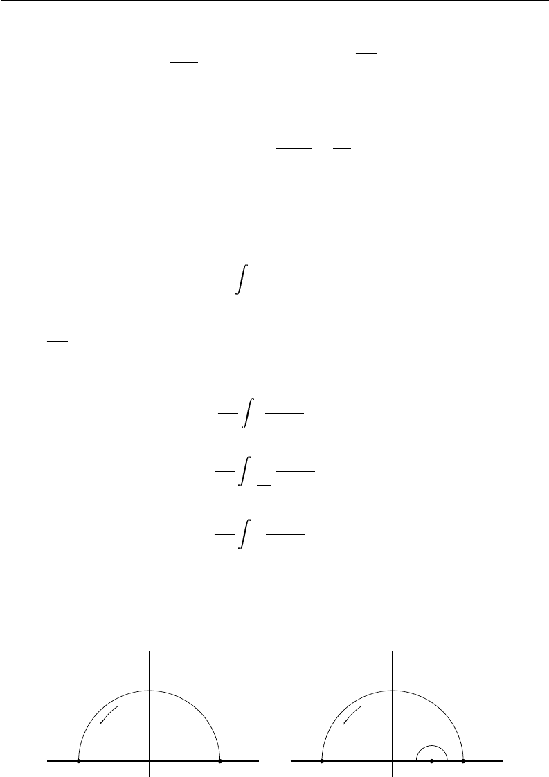
: |ρ| < R} (see fig. 2.8.1). By Cauchy’s integral
formula [14, p.84],
lnγ(ρ) =
1
2πi
C
R
lnγ(ξ)
ξ −ρ
dξ, ρ ∈ D
R
.
Since
lim
R→∞
1
2πi
|ξ|=R
ξ∈
Ω
+
lnγ(ξ)
ξ −ρ
dξ = 0,
we
obtain
lnγ
(ρ) =
1
2πi
∞
−∞
lnγ(ξ)
ξ −ρ
dξ, ρ ∈ Ω
+
. (2.8.51)
2)
T
ake a real σ and the closed contour C
σ
R,δ
(with counterclockwise circuit) consisting
of the semicircles C
0
R
= {ξ : ξ = Rexp(iϕ), ϕ ∈ [0, π]}, Γ
σ
δ
= {ξ : ξ−σ = δexp(iϕ), ϕ ∈
[0,π]}, δ > 0 and the intervals [−R,R] \[σ −δ, σ + δ] (see fig. 2.8.1).
6
-
6
-
/
ª
−R
R
6
-
6
-
/
ª
−R
R
σ
Figure
2.8.1.

140 G.
Freiling and V. Yurko
By Cauch
y’s theorem,
1
2πi
C
σ
R,δ
lnγ(ξ)
ξ −σ
dξ = 0.
Since
lim
R→∞
1
2πi
C
0
R
lnγ(ξ)
ξ −σ
dξ = 0, lim
δ→0
1
2πi
Γ
σ
δ
lnγ(ξ)
ξ −σ
dξ = −
1
2
lnγ(σ),
we
get
for real σ,
lnγ(σ) =
1
πi
∞
−∞
lnγ(ξ)
ξ −σ
dξ. (2.8.52)
In
(2.8.52)
(and everywhere below where necessary) the integral is understood in the prin-
cipal value sense.
3) Let γ(σ) = |γ(σ)|exp(−iβ(σ)). Separating in (2.8.52) real and imaginary parts we
obtain
β(σ) =
1
π
∞
−∞
ln|γ(ξ)|
ξ −σ
dξ, ln|γ(σ))| = −
1
π
∞
−∞
β(ξ)
ξ −σ
dξ.
Then,
using
(2.8.51) we calculate for ρ ∈ Ω
+
:
lnγ(ρ) =
1
2πi
∞
−∞
ln|γ(ξ)|
ξ −ρ
dξ −
1
2π
∞
−∞
β(ξ)
ξ −ρ
dξ
=
1
2πi
∞
−∞
ln|γ(ξ)|
ξ −ρ
dξ −
1
2π
2
∞
−∞
³
∞
−∞
dξ
(ξ −ρ)(s −ξ)
´
ln|γ(s)|d
s.
Since
1
(ξ −ρ)
(s −ξ
)
=
1
s −ρ
³
1
ξ −ρ
−
1
ξ −s
´
,
it
follo
ws that for ρ ∈ Ω
+
and real s,
∞
−∞
dξ
(ξ −ρ)(s −ξ)
=
πi
s −ρ
.
Consequently
,
lnγ
(ρ) =
1
πi
∞
−∞
ln|γ(ξ)|
ξ −ρ
dξ, ρ ∈ Ω
+
,
and
we
arrive at (2.8.50). 2
It follows from (2.8.21) and (2.8.26) that for real ρ 6= 0,
1
|a(ρ)|
2
= 1 −
|s
±
(ρ
)|
2
.
By virtue of (2.8.40) this yields for real ρ 6= 0,
|γ(ρ)| =
q
1 −
|s
±
(ρ
)|
2
.
Using (2.8.40) and (2.8.50) we obtain for ρ ∈ Ω
+
:
a(ρ) =
N
∏
k=1
ρ −iτ
k
ρ + iτ
k
e
xp
³
−
1
2πi
∞
−∞
ln(1 −
|s
±
(ξ)|
2
)
ξ −ρ
dξ
´
. (2.8.53)

Hyperbolic P
artial Differential Equations 141
We
note that since the function ρa(ρ) is continuous in
Ω
+
, it follo
ws that
ρ
2
1 −
|s
±
(ρ
)|
2
= O(1) as |ρ| → 0.
Relation (2.8.53) allows one to establish connections between the scattering data J
+
and J
−
. More precisely, from the given data J
+
one can uniquely reconstruct J
−
(and
vice versa) by the following algorithm.
Algorithm 2.8.1. Let J
+
be given. Then
1) construct the function a(ρ) by (2.8.53);
2) calculate d
k
and α
−
k
, k =
1,N by
(2.8.32);
3)
find b(ρ) and s
−
(ρ) by (2.8.26).
2. Solution of the inverse scattering problem
The inverse scattering problem is formulated as follows: given the scattering data J
+
(or J
−
), construct the potential q.
The central role for constructing the solution of the inverse scattering problem is played
by the so-called main equation which is a linear integral equation of Fredholm type. We
give a derivation of the main equation and study its properties. Using the main equation we
provide the solution of the inverse scattering problem along with necessary and sufficient
conditions of its solvability.
Theorem 2.8.5. For each fixed x, the functions A
±
(x,t), defined in (2.8.8) , satisfy
the integral equations
F
+
(x + y) + A
+
(x,y) +
∞
x
A
+
(x,t)F
+
(t + y)dt = 0, y > x, (2.8.54)
F
−
(x + y) + A
−
(x,y) +
x
−∞
A
−
(x,t)F
−
(t + y)dt = 0, y < x, (2.8.55)
where
F
±
(x) = R
±
(x) +
N
∑
k=1
α
±
k
exp(∓τ
k
x), (2.8.56)
and the functions R
±
(x) are defined by (2.8.28) .
Equations (2.8.54) and (2.8.55) are called the main equations or Gelfand-Levitan-
Marchenko equations for the inverse scattering problem.
Proof. By virtue of (2.8.18) and (2.8.19),
µ
1
a(ρ)
−1
g(x,ρ)
= s
+
(ρ
)e(x,ρ) + e(x,−ρ) −g(x,ρ). (2.8.57)
Put A
+
(x,t) = 0 for t < x, and A
−
(x,t) = 0 for t > x. Then, using (2.8.8) and (2.8.29),
we get
s
+
(ρ)e(x,ρ) + e(x,−ρ) −g(x,ρ)