Graef M. Introduction to conventional transmission electron microscopy

Подождите немного. Документ загружается.

98 Basic quantum mechanics

(a) (b)

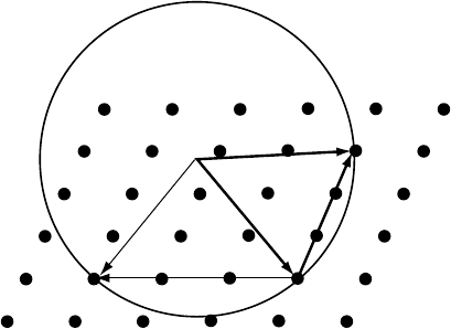
Fig. 2.3. (a) Geometrical construction leading to the reciprocal space Bragg equation; (b)

the diffracted wave vector is translated to complete the vector sum k



= k +g.

2.4.2 The Bragg equation in reciprocal space

We have already seen in Section 2.2.4 that a plane wave can be represented by its

momentum vector p, or, using the de Broglie relation, by its wave vector k. k is a

vector in reciprocal space which fully characterizes the direction and wavelength

of a plane wave with respect to the crystal reference frame. Since the plane (hkl)is

also represented by a vector g

hkl

in reciprocal space, we can derive the reciprocal

space equivalent of the Bragg equation (2.40).

Consider the drawing in Fig. 2.3(a). It shows the wave vectors corresponding

to the incident and diffracted wave directions of Fig. 2.2(a). The reciprocal lattice

vector g

hkl

is also drawn in the proper orientation. Since vectors can always be

translated parallel to themselves, we can redraw the diffracted vector k



so that its

starting point coincides with the starting point C of k, as shown in Fig. 2.3(b). The

relation between the three vectors can now be expressed as



= k + g. (2.41)

Note that the length of the wave vectors is constant for elastic scattering processes.

It is easy to see that this vector relation is equivalent to the direct space Bragg

equation (2.40). Projecting the above equation onto the vector g leads to



· g = k ·g + g · g;

|k||g|sin θ =−|k||g|sin θ +|g|

;

sin θ

=−

sin θ

hkl

from which the Bragg equation follows. The Bragg relation is thus satisﬁed when-

ever the point C in Fig. 2.3(b) falls on the perpendicular bisector plane of the

vector g.

2.4 The Bragg equation in direct and reciprocal space 99

Ewald

sphere

k''

Fig. 2.4. Ewald sphere construction.

The perpendicular bisector plane to the vector g

hkl

consists of all the points

that are at the same distance from the origin of reciprocal space and the re-

ciprocal lattice point hkl. This leads to a simple geometric construction for the

direction of a diffracted wave, when the incident wave vector and the crystal

orientation are given. The construction is known as the Ewald sphere construc-

tion and is shown in Fig. 2.4. First draw the reciprocal lattice with origin O.

Then draw the incident wave vector k such that its end point coincides with

O. The starting point C is then taken to be the center of a sphere (the Ewald

sphere) with radius |k|=1/λ. Whenever a reciprocal lattice point falls on this

sphere, the Bragg condition is satisﬁed and a diffracted wave with wave vector

k + g may occur.

†

Note that there are two reciprocal lattice points on the Ewald

sphere in Fig. 2.4; this means that there are two diffracted beams in the directions



and k



Recall from the de Broglie relation that the momentum vector and the wave

vector are identical, apart from a scaling factor h. The Bragg equation in reciprocal

space can thus be rewritten as



= p + hg = p + p. (2.42)

This equation reﬂects the fact that the incident electron with momentum p under-

goes a change of direction corresponding to hg. Reciprocal lattice vectors thus

correspond to the allowed elastic momentum changes (in units of Planck’s con-

stant) for a given crystal structure.

‡

It is somewhat surprising that the allowed

momentum changes for elastic scattering do not depend on the energy or type of

†

Note that we say “may occur”, because the Bragg equation only states the geometrical condition for diffraction.

As we shall see later on, this does not necessarily mean that there will be diffracted intensity in that direction.

‡

It is easy to verify that hg indeed has the dimensions of momentum.

100 Basic quantum mechanics

incident radiation, but are determined entirely by the crystal structure. We ﬁnd that

the reciprocal lattice not only provides us with a way to describe crystal planes and

interplanar spacings, it also determines the allowed momentum changes for elastic

scattering events.

Example 2.1 Compute the momentum transfer for elastic scattering of an electron

from the (220) planes in aluminum.

Answer: The lattice parameter of face-centered cubic aluminum is a = 0.4049 nm

[VC85]. From the relations derived in Chapter 1 we ﬁnd for the length of the vector

220

: |g

220

√

8/a = 6.9855 nm

−1

. Multiplying by Planck’s constant then results

in the elastic momentum transfer p = 4.628 × 10

−24

kg m s

−1

It can be seen from the Ewald sphere construction that diffraction is a rather

improbable process. It requires that a mathematical point (with zero volume) should

fall on to a spherical shell of zero thickness. For real crystals and for realistic types

of radiation we will see that the reciprocal lattice point occupies a ﬁnite volume with

a well-deﬁned shape, and that the Ewald sphere has a ﬁnite thickness related to the

wavelength spread of the radiation. These two factors combine to make diffraction

a much more probable process. In almost all diffraction experiments one has the

ability to either move the incident beam direction (which corresponds to moving the

Ewald sphere through the reciprocal lattice), or move the crystal with a stationary

incident beam direction (which corresponds to moving the reciprocal lattice through

the Ewald sphere). In a transmission electron microscope both options are present:

we can change the incident beam direction within a small range of directions using

beam tilt controls and the sample can be tilted around one or more axes, so that the

orientation of the crystal lattice with respect to the incident beam direction can be

changed.

2.4.3 The geometry of electron diffraction

It will be useful to have a mathematical expression for the Ewald sphere. The

general equation of a sphere can be written down in vector form as follows:

(r − r

) · (r − r

) = R

where R is the radius and r

is the vector locating the center of the sphere. This

equation is valid in every reference frame, and in the simple case of the Cartesian

frame we recover the standard equation

(x − x

)

+ (y − y

)

+ (z − z

)

= R

2.4 The Bragg equation in direct and reciprocal space 101

2k+q

>90

<90

(a)

k+k'

Perpendicular

bisector plane

(b)

Fig. 2.5. (a) Illustration of the vector equation (2.43) for the Ewald sphere; (b) Bragg

orientation for the planes g.

In reciprocal space we replace the position vector r by a reciprocal space vector q;

the center of the Ewald sphere is located at the position given by the vector −k,

and the radius is equal to the inverse of the wavelength R = 1/λ. This leads to

(q + k) · (q + k) =

Since |k|=1/λ we can rewrite this equation as

q · (2k + q) = 0. (2.43)

This is the equation for the Ewald sphere: every vector q that is perpendicular to

the vector 2k + q must end on the Ewald sphere. The dot product is negative when

q ends inside the Ewald sphere, and positive when it ends outside the sphere, as

can be seen from Fig. 2.5(a). The Bragg equation in reciprocal space can therefore

be rewritten for a given reciprocal lattice vector g as

g · (2k + g) = g · (k + k



) = 0.

This relation expresses the fact that the bisector plane of g must contain the vector

k + k



for the exact Bragg orientation, as shown in Fig. 2.5(b).

Fig. 2.6 shows the diffraction angle 2θ (in mrad)

†

for the (200), (400), and

(600) lattice planes in aluminum (a = 0.4049 nm) as a function of the acceleration

voltage E (log–linear plot). The vertical lines indicate the commonly used voltages

†

Recall that 1 mrad equals 0.057 2958

◦

= 3





102 Basic quantum mechanics

Table 2.3. Diffraction angles 2θ for the (200), (400), and (600) lattice

planes in aluminum for E = 200 kV and E = 1 MV in mrad (degrees).

The last column shows the corresponding angles for x-ray diffraction

using Cu-K

radiation with λ = 0.154 2838 nm; the (600) planes do not

give rise to a diffracted beam for this wavelength.

Plane 2θ

200 kV

2θ

1MeV

Cu-K

x-rays

(200) 12.38 (0.71) 4.31 (0.25) 781.31 (44.76)

(400) 24.77 (1.42) 8.61 (0.49) 1731.52 (99.21)

(600) 37.16 (2.13) 12.92 (0.74) —

Accelerating

Voltage E [Volts]

Diffraction Angle 2θ [mrad]

200 kV 1 MV

10 10

(200)

(400)

(600)

Fig. 2.6. Log–linear plot of the diffraction angle 2θ (mrad) versus acceleration voltage E

(volts) for the (200), (400), and (600) lattice planes in aluminum.

E = 200 kV and E = 1 MV. Table 2.3 lists the corresponding diffraction angles

2θ in mrad and degrees, computed using

2θ

hkl

= 2 sin

−1



hkl



For comparison, the table also shows the diffraction angle for diffraction using

Cu-K

x-rays. It can be seen from the table that it is a good approximation to

replace sin θ by θ for electron diffraction, since the diffraction angles increase

nearly linearly with |g

hkl

Table 2.2 on page 93 lists the length of the wave vector K

(or, equivalently, the

radius of the Ewald sphere) for the commonly used acceleration voltages. Note that

these numbers are two to three orders of magnitude larger than the typical length of

a reciprocal lattice vector g

hkl

. This means that the Ewald sphere has a large radius

2.5 Fourier transforms and convolutions 103

200 keV

1 MeV

2.5 nm

--1

Fig. 2.7. Ewald sphere drawn to scale for the reciprocal lattice of a square crystal with

lattice parameter 0.4 nm, and a 200 keV and 1 MeV incident electron beam.

compared to the dimensions of the reciprocal lattice. Near the origin of reciprocal

space the Ewald sphere is nearly planar, as shown in Fig. 2.7, which represents a to-

scale drawing of a square reciprocal lattice with lattice parameter a

∗

= 2.5nm

−1

The Ewald spheres corresponding to acceleration voltages of 200 kV and 1 MV

are superimposed on the drawing. The radii of the Ewald spheres (on the scale of

the drawing) are 340 and 977 mm, respectively, for 200 and 1000 kV electrons.

Diffracted beams are therefore nearly parallel to the incident beam, with diffraction

angles 2θ of the order of a degree or so. Diffraction of high-energy electrons is then

essentially a forward-scattering process, and most electron trajectories are oriented

at small angles with respect to the incident beam.

2.5 Fourier transforms and convolutions

2.5.1 Deﬁnition

Consider a particle described by a wave function (r). In general, this function will

be a superposition of different momentum eigenstates, each with its own momentum

eigenvalue p. Since we have established the relation between p and k, we will

continue to use the wave vector description from here on. Suppose we ask the

question: how much does a certain wave vector k contribute to this function (r)?

In other words, if  is written as a superposition of momentum eigenfunctions,

then what is the weight (k) of the eigenfunction with wave vector k?

This question is answered readily by considering the analogy with vectors: given

a vector t, what is the contribution of the basis vector e

to t? We know that the

components of a vector can be determined by projecting this vector onto the three

basis vectors, so we ﬁnd:

t · e

(

+ ve

+ we

)

· e

= u.

The dot product thus allows us to determine the components (or projection) of

a vector with respect to a set of basis vectors. All we need to determine those

components is a set of independent (basis) vectors e

104 Basic quantum mechanics

The dot product can also be deﬁned for continuous functions, as we have seen in

Section 2.2.1, and if we apply equation (2.2) to the unit amplitude plane wave we

ﬁnd

2πik·r

2πik



·r

...

2πi(k



−k)·r

dr = δ(k



− k).

Now we are ready to answer the question posed at the beginning of this section:

the contribution of the wave vector k to the wave function (r) is determined from

the projection of (r) onto the momentum eigenfunction corresponding to k:

(k) =

2πik·r

(r)

. (2.44)

We thus have an integral relation between the functions (r) and (k), which is

given explicitly by

(k) =

...

−2πik·r

(r)dr.

We deﬁne the direct Fourier transform (DFT) of the function (r)as

(k) = F[(r)] ≡

...

(r)e

−2πik·r

dr, (2.45)

where the integral extends over all of 3D space. The operator F represents the DFT.

The inverse Fourier transform (IFT) is then deﬁned by

(r) = F

−1

[(k)] ≡

...

(k)e

2πik·r

dk. (2.46)

The Fourier transform thus establishes a mechanism for converting a direct space

wave function into its reciprocal space equivalent, which is essentially a momentum

space representation of that function (apart from a constant scaling factor). We will

represent the DFT of a function by a function with the same symbol, but with a

reciprocal vector as its argument; in other words, the functions (r) and (k) form

a Fourier transform pair.

At this point we should warn the reader that there are a few different notational

systems around in the literature (see [Spe88, pp. 155–156] and [VAJ99, pp. 333–

338] for a comparative list of notations, and a discussion of the history of the two

conventions). First of all, it is possible to change the order of the functions in

equation (2.44); this means that the sign of the exponent of the DFT will change

to positive instead of negative, and the IFT will now have the minus sign (this is

known as the crystallographic sign convention). Both conventions are in use, and

the reader should be careful in comparing expressions from various textbooks. In

addition, solid-state physicists often incorporate the factor of 2π in the deﬁnition

2.5 Fourier transforms and convolutions 105

of the wave vector, i.e. |k|=2π/λ; in other words, they scale reciprocal space by

a factor of 2π. The reciprocal basis vectors, deﬁned in equation (1.9) on page 11,

must then also be multiplied by 2π , and the de Broglie relation then contains the

factor h

instead of h. Finally, the factor of 2π is sometimes put in front of both

Fourier integrals, in the form 1/(2π)

D/2

, where D is the dimensionality of the

space in which the transform is computed. Hence, when comparing formulas in

the literature, be aware of the fact that the Fourier transform can be deﬁned in

several different ways, all of which are correct, provided subsequent calculations

are performed in a consistent way. For an in-depth study of Fourier transforms and

related mathematical operations as applied to diffraction phenomena we refer the

reader to [Don69], [BW75], [Cow81], and [Bra86]. In this book, we will adhere to

the quantum mechanical sign convention, which has a minus sign in the exponential

of the direct Fourier transform.

2.5.2 The Dirac delta-function

The Dirac delta-function is a rather strange mathematical object which seems to

defy normal properties of continuity and differentiability and still remains useful

in various types of integral calculations. Although there is a rigorous mathematical

deﬁnition of this and related functions in the theory of distributions [Don69, pp. 91–

96], we will restrict ourselves to some simple deﬁnitions and properties (see, e.g.,

[Bra86]).

The Dirac δ-function is deﬁned by

δ(r − a) =

0 r = a;

∞ r = a.

(2.47)

It is represented by an inﬁnitely narrow peak of inﬁnite height at the position r = a,

with the additional property that the area under the peak is equal to one:

...

δ(r − a)dr = 1. (2.48)

If we multiply the δ-function by a constant c, then the function cδ(r − a)isa

delta-function of weight c.

We can regard the δ-function as the limiting case of the Gaussian distribution,

when the width of the distribution goes to zero and the amplitude to inﬁnity, keeping

the area under the curve normalized; in the 1D case this is described by

δ(x) = lim

a→∞



√

−a



. (2.49)

106 Basic quantum mechanics

Another useful property is the complex representation of the delta-function:

δ(k) = F[1] =

...

−2πik·r

dr. (2.50)

Comparing this relation to the deﬁnition of the DFT, we ﬁnd that the Fourier

transform of the constant 1 is equal to δ(k). The Fourier transform of a constant c

is a δ-function of weight c (F[c] = cF[1] = cδ(k)).

2.5.3 The convolution product

The convolution product C(r) (also known as folding or faltung) of two functions

f (r) and g(r) is deﬁned by

C(r) ≡ f (r) ⊗ g(r) =

...

f (R)g(r − R)dR. (2.51)

The Dirac δ-function is the identity operator of the convolution product:

f (r) ⊗ δ(r) =

...

f (R)δ(r − R)dR = f (r). (2.52)

This is known as the sifting property of the δ-function. The following two theorems

are useful:

the multiplication theorem: F[ f (r)g(r)] = F(k) ⊗ G(k); (2.53)

the convolution theorem: F[ f (r) ⊗ g(r)] = F(k)G(k). (2.54)

The proof for these theorems is quite straightforward and is left to the reader (see,

e.g., [Cow81]).

Convolutions are fundamental to many different types of experiments. In a rather

general sense, we can describe an experiment as follows: a reference signal R is

created and directed at the material to be investigated. This could be a beam of

electrons, or monochromatic light, or a heat pulse, or anything else. The sample then

modiﬁes this reference signal, and ideally we would like to measure the modiﬁed

signal R



. In practice, however, the detector system, which converts the modiﬁed

signal into an observable signal (e.g. visible light, or an electrical current or voltage)

introduces its own ﬁngerprint onto the signal R



. In the simplest case this would be

a linear scaling of R



, but in many cases the relationship between detected signal



and modiﬁed signal R



is non-linear and can be described by a convolution of



with a function T , known as the instrument point spread function:



= T ⊗ R



. (2.55)

2.5 Fourier transforms and convolutions 107

Fig. 2.8. Illustration of the convolution product of two functions. The function on the second

row is broader than on the ﬁrst row, and the resulting convolution product signiﬁcantly

reduces (blurs) the high-frequency detail of the original function.

Almost invariably, this means that the instrument imposes a resolution limit, which

results in blurring of the smallest details in the signal R



. An example of such

blurring is shown in Fig. 2.8, which shows the convolution of a high-frequency

signal with two point spread functions, one narrow and the other wide. The high-

frequency details are suppressed by the convolution with the wider point spread

function.

We have seen above that the Dirac delta-function is the identity operator for the

convolution product, so it follows that for an ideal instrument, i.e. one that does

not leave its ﬁngerprint on the modiﬁed signal, the point spread function should

be equal to the Dirac delta-function. In the case of electron microscopy, it is the

task of the microscope manufacturer to design a detector system (which includes

all microscope lenses and the viewing screen or camera) that has a minimal im-

pact on the modiﬁed signal R



. We will see in later chapters that this is only

partially possible and as microscope users we need to be aware of how the micro-

scope affects the wave function of the electrons after they have passed through the

sample.

One might think that if the function T were fully known, then a measurement of



, followed by a mathematical operation known as deconvolution, would yield the

function R



directly. Using the convolution theorem we can reconstruct the signal

function as:



= F

−1



F[R



]

F[T ]



. (2.56)

It is obvious that this deconvolution procedure only works when F[T ] does not

contain any zeros. As we will see in the chapter on phase contrast microscopy