Greene W.H. Econometric Analysis

Подождите немного. Документ загружается.

CHAPTER 19

✦

Limited Dependent Variables

839

which is a function of x

. If we estimate (19-10) by ordinary least squares regression of

y on X, then we have omitted a variable, the nonlinear term λ

. All the biases that arise

because of an omitted variable can be expected.

Without some knowledge of the distribution of x, it is not possible to determine

how serious the bias is likely to be. A result obtained by Chung and Goldberger

(1984) is broadly suggestive. If E [x | y] in the full population is a linear function of

y, then plim b = βτ for some proportionality constant τ . This result is consistent with

the widely observed (albeit rather rough) proportionality relationship between least

squares estimates of this model and maximum likelihood estimates.

The proportional-

ity result appears to be quite general. In applications, it is usually found that, compared

with consistent maximum likelihood estimates, the OLS estimates are biased toward

zero. (See Example 19.5.)

19.2.4 THE STOCHASTIC FRONTIER MODEL

A lengthy literature commencing with theoretical work by Knight (1933), Debreu

(1951), and Farrell (1957) and the pioneering empirical study by Aigner, Lovell, and

Schmidt (ALS, 1977) has been directed at models of production that speciﬁcally ac-

count for the textbook proposition that a production function is a theoretical ideal.

y = f (x) deﬁnes a production relationship between inputs, x, and an output, y, then for

any given x, the observed value of y must be less than or equal to f (x). The implication

for an empirical regression model is that in a formulation such as y = h(x, β) + u, u

must be negative. Because the theoretical production function is an ideal—the frontier

of efﬁcient production—any nonzero disturbance must be interpreted as the result of in-

efﬁciency. A strictly orthodox interpretation embedded in a Cobb–Douglas production

model might produce an empirical frontier production model such as

ln y = β



ln x

− u, u ≥ 0.

The gamma model described in Example 4.7 was an application. One-sided distur-

bances such as this one present a particularly difﬁcult estimation problem. The primary

theoretical problem is that any measurement error in ln y must be embedded in the

disturbance. The practical problem is that the entire estimated function becomes a slave

to any single errantly measured data point.

Aigner, Lovell, and Schmidt proposed instead a formulation within which observed

deviations from the production function could arise from two sources: (1) productive

inefﬁciency, as we have deﬁned it earlier and that would necessarily be negative, and

(2) idiosyncratic effects that are speciﬁc to the ﬁrm and that could enter the model with

either sign. The end result was what they labeled the stochastic frontier:

ln y = β



ln x

− u + v, u ≥ 0,v∼ N



0,σ



= β



ln x

+ ε.

See Heckman (1979) who formulates this as a “speciﬁcation error.”

See the appendix in Hausman and Wise (1977) and Greene (1983) as well.

A survey by Greene (2008a) appears in Fried, Lovell, and Schmidt (2008). Kumbhakar and Lovell (2000) is

a comprehensive reference on the subject.

840

PART IV

✦

Cross Sections, Panel Data, and Microeconometrics

The frontier for any particular ﬁrm is h(x, β)+v, hence the name stochastic frontier.The

inefﬁciency term is u, a random variable of particular interest in this setting. Because

the data are in log terms, u is a measure of the percentage by which the particular

observation fails to achieve the frontier, ideal production rate.

To complete the speciﬁcation, they suggested two possible distributions for the in-

efﬁciency term: the absolute value of a normally distributed variable, which has the

truncated at zero distribution shown in Figure 19.1, and an exponentially distributed

variable. The density functions for these two compound variables are given by Aigner,

Lovell, and Schmidt; let ε = v − u,λ = σ

/σ

,σ = (σ

+ σ

)

1/2

, and (z) =the prob-

ability to the left of z in the standard normal distribution (see Section B.4.1). For the

“half-normal” model,

ln h(ε

|β,λ,σ) =



−ln σ +





−





+ ln 



−ε



whereas for the exponential model

ln h(ε

|β,θ,σ

) =



ln θ +

+ θε

+ ln 



−

− θσ



Both these distributions are asymmetric. We thus have a regression model with a

nonnormal distribution speciﬁed for the disturbance. The disturbance, ε, has a nonzero

mean as well; E [ε] =−σ

(2/π)

1/2

for the half-normal model and −1/θ for the expo-

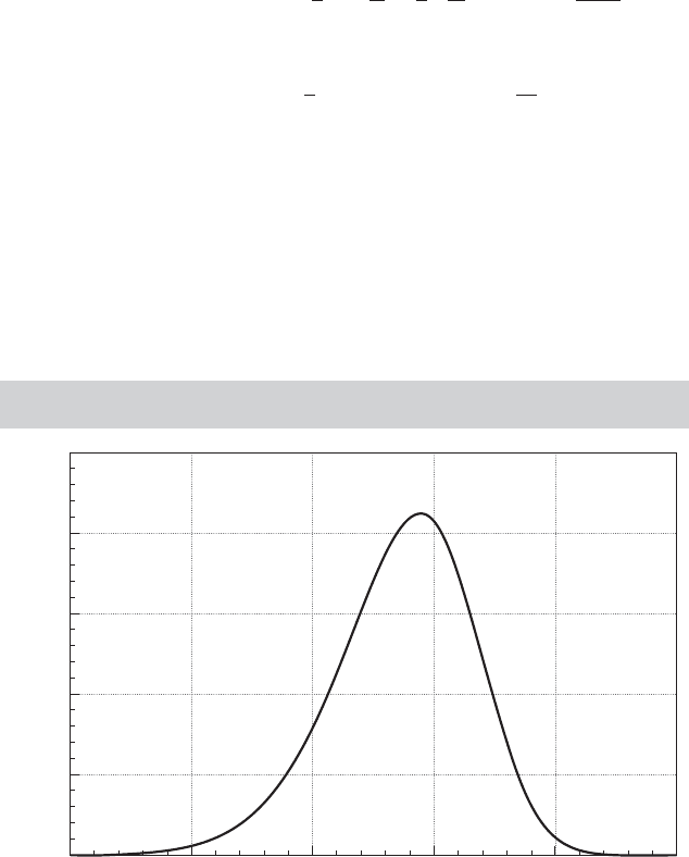
nential model. Figure 19.2 illustrates the density for the half-normal model with σ = 1

and λ = 2. By writing β

= β

+E [ε] and ε

∗

= ε −E [ε], we obtain a more conventional

formulation

ln y = β



ln x

+ ε

∗

FIGURE 19.2

Density for the Disturbance in the Stochastic Frontier

Model.

2.8 1.6

Density

0.4

␧

0.8 2.04.0

0.00

0.70

0.56

0.42

0.28

0.14

CHAPTER 19

✦

Limited Dependent Variables

841

which does have a disturbance with a zero mean but an asymmetric, nonnormal distribu-

tion. The asymmetry of the distribution of ε

∗

does not negate our basic results for least

squares in this classical regression model. This model satisﬁes the assumptions of the

Gauss–Markov theorem, so least squares is unbiased and consistent (save for the con-

stant term) and efﬁcient among linear unbiased estimators. In this model, however, the

maximum likelihood estimator is not linear, and it is more efﬁcient than least squares.

The log-likelihood function for the half normal model is given in ALS (1977):

ln L =−n ln σ +

−



i=1







i=1

ln 



−ε



. (19-11)

Maximization programs for this model are built into modern software packages such as

Stata, NLOGIT, and TSP. The log-likelihood is simple enough that it can also be readily

adapted to the generic optimization routines in, for example, MatLab or Gauss. Some

treatments in the literature use the parameterization employed by Battese and Coelli

(1992) and Coelli (1996), γ = σ

/σ

. This is a one-to-one transformation of λ;λ =

(γ /(1 − γ))

1/2

, so which parameterization is employed is a matter of convenience; the

empirical results will be the same. The log-likelihood function for the exponential model

can be built up from the density given earlier. For the half-normal model, we would also

rely on the invariance of maximum likelihood estimators to recover estimates of the

structural variance parameters, σ

= σ

/(1 + λ

) and σ

= σ

/(1 + λ

(Note, the

variance of the truncated variable,u

,isnotσ

; using (19-2), it reduces to (1−2/π)σ

].) In

addition, a structural parameter of interest is the proportion of the total variance of ε that

is due to the inefﬁciency term. For the half-normal model, Var[ε] = Var[u] + Var[v] =

(1 − 2/π)σ

+ σ

whereas for the exponential model, the counterpart is 1/θ

+ σ

Modeling in the stochastic frontier setting is rather unlike what we are accustomed

to up to this point, in that the disturbance, speciﬁcally u

, not the model parameters, is

the central focus of the analysis. The reason is that in this context, the disturbance, u

rather than being the catchall for the unknown and unknowable factors omitted from

the equation, has a particular interpretation—it is the ﬁrm-speciﬁc inefﬁciency. Ideally,

we would like to estimate u

for each ﬁrm in the sample to compare them on the basis

of their productive efﬁciency. Unfortunately, the data do not permit a direct estimate,

because with estimates of β in hand, we are only able to compute a direct estimate of

= y

−x



β. Jondrow et al. (1982), however, have derived a useful approximation that

is now the standard measure in these settings,

E[u

|ε

] =

σλ

1 + λ



φ(z

)

1 − (z

)

− z



, z

for the half-normal model, and

E[u

|ε

] = z

+ σ

φ(z

/σ

)

(z

/σ

)

, z

=−



+ θσ



for the exponential model.These values can be computed using the maximum likelihood

estimates of the structural parameters in the model. In some cases in which researchers

A vexing problem for estimation of the model is that if the ordinary least squares residuals are skewed in

the positive (wrong) direction (See Figure 19.2), OLS with

λ = 0 will be the MLE. OLS residuals with a

positive skew are apparently inconsistent with a model in which, in theory, they should have a negative skew.

[See Waldman (1982) for theoretical development of this result.]

842

PART IV

✦

Cross Sections, Panel Data, and Microeconometrics

are interested in discovering best practice [e.g., WHO (2000), Tandon et al. (2000)], the

estimated values are sorted and the ranks of the individuals in the sample become of

interest.

Research in this area since the methodological developments beginning in the 1930s

and the building of the empirical foundations in 1977 and 1982 has proceeded in several

directions. Most theoretical treatments of “inefﬁciency” as envisioned here attribute

it to aspects of management of the ﬁrm. It remains to establish a ﬁrm theoretical con-

nection between the theory of ﬁrm behavior and the stochastic frontier model as a

device for measurement of inefﬁciency.

In the context of the model, many studies have developed alternative, more ﬂexible

functional forms that (it is hoped) can provide a more realistic model for inefﬁciency.

Two that are relevant in this chapter are Stevenson’s (1980) truncated normal model

and the normal-gamma frontier. One intuitively appealing form of the truncated normal

model is

∼ N



μ + z



α,σ



=|U

The original normal–half-normal model results if μ equals zero and α equals zero. This

is a device by which the environmental variables noted in the next paragraph can enter

the model of inefﬁciency. A truncated normal model is presented in Example 19.3. The

half-normal, truncated normal, and exponential models all take the form of distribution

shown in Figure 19.1. The gamma model,

f (u) = [θ

/(P)] exp(−θ u)u

P−1

is a ﬂexible model that presents the advantage that the distribution of inefﬁciency

can move away from zero. If P is greater than one, then the density at u = 0 equals

zero and the entire distribution moves away from the origin. The implication is that

the distribution of inefﬁciency among ﬁrms can move away from zero. The gamma

model is estimated by simulation methods—either Bayesian MCMC [Huang (2003)

and Tsionas (2002)] or maximum simulated likelihood [Greene (2003)]. Many other

functional forms have been proposed. [See Greene (2008) for a survey.]

There are usually elements in the environment in which the ﬁrm operates that

impact the ﬁrm’s output and/or costs but are not, themselves, outputs, inputs, or input

prices. In Example 19.3, the costs of the Swiss railroads are affected by three variables;

track width, long tunnels, and curvature. It is not yet speciﬁed how such factors should be

incorporated into the model; four candidates are in the mean and variance of u

, directly

in the function, or in the variance of v

. [See Hadri, Guermat, and Whittaker (2003) and

Kumbhakar (1997c).] All of these can be found in the received studies. This aspect of

the model was prominent in the discussion of the famous World Health Organization

efﬁciency study of world health systems [WHO (2000), Tandon, Murray, Lauer, and

Evans (2000), and Greene (2004)]. In Example 19.3, we have placed the environmental

factors in the mean of the inefﬁciency distribution. This produces a rather extreme

set of results for the JLMS estimates of inefﬁciency—many railroads are estimated

to be extremely inefﬁcient. An alternative formulation would be a “heteroscedastic”

model in which σ

u,i

= σ

exp(z



δ) or σ

v,i

= σ

exp(z



η), or both. We can see from the

JLMS formula that the term heteroscedastic is actually a bit misleading, since both

CHAPTER 19

✦

Limited Dependent Variables

843

standard deviations enter (now) λ

, which is, in turn, a crucial parameter in the mean

of inefﬁciency.

How should inefﬁciency be modeled in panel data, such as in our example? It

might be tempting to treat it as a time-invariant “effect” [as in Schmidt and Sickles

(1984) and Pitt and Lee (1984) in two pioneering papers]. Greene (2004) argued that a

preferable approach would be to allow inefﬁciency to vary freely over time in a panel,

and to the extent that there is a common time-invariant effect in the model, that should

be treated as unobserved heterogeneity, not inefﬁciency. A string of studies, including

Battese and Coelli (1992, 1995), Cuesta (2000), Kumbhakar (1997a) Kumbhakar and

Orea (2004), and many others have proposed hybrid forms that treat the core random

part of inefﬁciency as a time-invariant ﬁrm-speciﬁc effect that is modiﬁed over time by

a deterministic, possibly ﬁrm-speciﬁc, function. The Battese-Coelli form,

= exp[−η(t − T)]|U

| where U



0,σ



has been used in a number of applications. Cuesta (2000) suggests allowing η to vary

across ﬁrms, producing a model that bears some relationship to a ﬁxed-effects speciﬁ-

cation. This thread of the literature is one of the most active ongoing pursuits.

Is it reasonable to use a possibly restrictive parametric approach to modeling in-

efﬁciency? Sickles (2005) and Kumbhakar, Simar, Park, and Tsionas (2007) are among

numerous studies that have explored less parametric approaches to efﬁciency analysis.

Proponents of data envelopment analysis [see, e.g., Simar and Wilson (2000, 2007)] have

developed methods that impose absolutely no parametric structure on the production

function. Among the costs of this high degree of ﬂexibility is a difﬁculty to include envi-

ronmental effects anywhere in the analysis, and the uncomfortable implication that any

unmeasured heterogeneity of any sort is necessarily included in the measure of inefﬁ-

ciency. That is, data envelopment analysis returns to the deterministic frontier approach

where this section began.

Example 19.3 Stochastic Cost Frontier for Swiss Railroads

Farsi, Filippini, and Greene (2005) analyzed the cost efﬁciency of Swiss railroads. In order to

use the stochastic frontier approach to analyze costs of production, rather than production,

we rely on the fundamental duality of production and cost [see Samuelson (1938), Shephard

(1953), and Kumbhakar and Lovell (2000)]. An appropriate cost frontier model for a ﬁrm that

produces more than one output—the Swiss railroads carry both freight and passengers—will

appear as the following:

ln(C/P

) = α +

K −1



k=1

ln( P

) +



m=1

ln Q

+ v + u.

The requirement that the cost function be homogeneous of degree one in the input prices

has been imposed by normalizing total cost, C, and the ﬁrst K −1 prices by the K th input

price. In this application, the three factors are labor, capital, and electricity—the third is

used as the numeraire in the cost function. Notice that the inefﬁciency term, u, enters the

cost function positively; actual cost is above the frontier cost. [The MLE is modiﬁed simply by

replacing ε

with −ε

in (19-11).] In analyzing costs of production, we recognize that there is an

additional source of inefﬁciency that is absent when we analyze production. On the production

side, inefﬁciency measures the difference between output and frontier output, which arises

because of technical inefﬁciency. By construction, if output fails to reach the efﬁcient level

for the given input usage, then costs must be higher than frontier costs. However, costs can

be excessive even if the ﬁrm is technically efﬁcient if it is “allocatively inefﬁcient.” That is, the

ﬁrm can be technically efﬁcient while not using inputs in the cost minimizing mix (equating

844

PART IV

✦

Cross Sections, Panel Data, and Microeconometrics

the ratio of marginal products to the input price ratios). It follows that on the cost side, “u”

can contain both elements of inefﬁciency while on the production side, we would expect to

measure only technical inefﬁciency. [See Kumbhakar (1997b).]

The data for this study are an unbalanced panel of 50 railroads with T

ranging from 1

to 13. (Thirty-seven of the ﬁrms are observed 13 times, 8 are observed 12 times, and the

remaining 5 are observed 10, 7, 7, 3, and 1 times.) The variables we will use here are

CT: Total costs adjusted for inﬂation (1,000 Swiss franc)

QP: Total passenger-output in passenger-kilometers

QF: Total goods-output in ton-kilometers

PL: Labor price adjusted for inﬂation (in Swiss Francs per person per year)

PK: Capital price with capital stock proxied by total number of seats

PE: Price of electricity (Swiss franc per kWh)

Logs of costs and prices (ln CT,lnPK,lnPL) are normalized by PE. We will also use these

environmental variables:

NARROW

T: Dummy for the networks with narrow track (1 m wide) The usual

width is 1.435m.

TUNNEL: Dummy for networks that have tunnels with an average length

of more than 300 meters.

VIRAGE: Dummy for the networks whose minimum radius of curvature is

100 meters or less.

The full data set is given in Appendix Table F19.1. Several other variables not used here are

presented in the appendix table. In what follows, we will ignore the panel data aspect of the

data set. This would be a focal point of a more extensive study.

There have been dozens of models proposed for the inefﬁciency component of the

stochastic frontier model. Table 19.1 presents several different forms. The basic half-normal

model is given in the ﬁrst column. The estimated cost function parameters across the different

TABLE 19.1

Estimated Stochastic Frontier Cost Functions

Model

Half Truncated

Variable Normal Normal Exponential Gamma Heterosced Heterogen

Constant −10.0799 −9.80624 −10.1838 −10.1944 −9.82189 −10.2891

ln QP 0.64220 0.62573 0.64403 0.64401 0.61976 0.63576

ln QF 0.06904 0.07708 0.06803 0.06810 0.07970 0.07526

ln PK 0.26005 0.26625 0.25883 0.25886 0.25464 0.25893

ln PL 0.53845 0.50474 0.56138 0.56047 0.53953 0.56036

Constant 0.44116 −2.48218

Narrow 0.29881 2.16264

0.14355

Virage −0.20738 −1.52964

−0.10483

Tunnel 0.01118 0.35748

−0.01914

σ 0.44240 0.38547 (0.34325) (0.34288) 0.45392

0.40597

λ 1.27944 2.35055 0.91763

P 1.0000 1.22920

θ 13.2922 12.6915

(0.34857) (0.35471) (0.07523) (0.09685) 0.37480

0.27448

(0.27244) (0.15090) 0.33490 0.33197 0.25606 0.29912

Mean E[u|ε] 0.27908 0.52858 0.075232 0.096616 0.29499 0.21926

ln L −210.495 −200.67 −211.42 −211.091 −201.731 −208.349

Estimates in parentheses are derived from other MLEs.

Estimates used in computation of σ

Obtained by averaging λ = σ

u,i

/σ

over observations.

CHAPTER 19

✦

Limited Dependent Variables

845

0.00 0.10 0.20 0.30 0.40 0.50 0.60 0.70 0.80 0.90

0.00

1.02

2.04

3.06

Density

4.08

5.10

Inefficiency

Heterogeneous

Half-Normal

Heteroscedastic

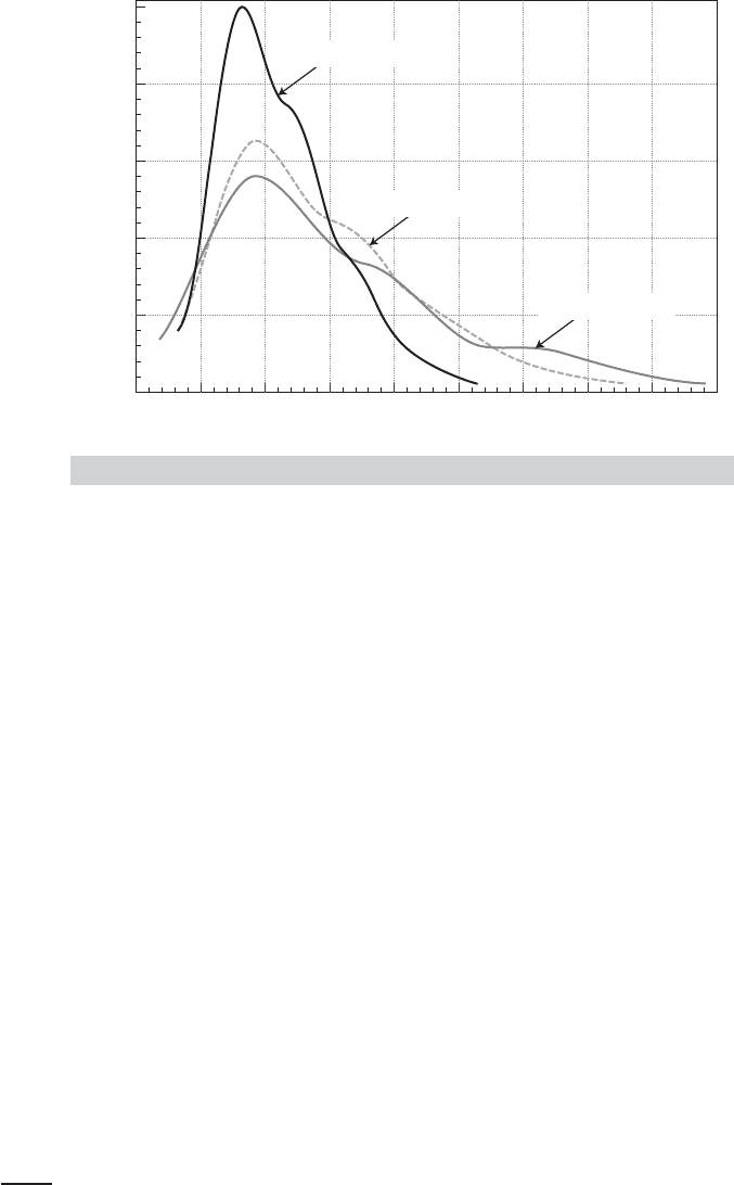
FIGURE 19.3

Kernel Density Estimator for JLMS Estimates.

forms are broadly similar, as might be expected as (α, β) are consistently estimated in all

cases. There are fairly pronounced differences in the implications for the components of ε,

however.

There is an ambiguity in the model as to whether modiﬁcations to the distribution of u

will affect the mean of the distribution, the variance, or both. The following results suggest

that it is both for these data. The gamma and exponential models appear to remove most

of the inefﬁciency from the data. Note that the estimates of σ

are considerably smaller

under these speciﬁcations, and σ

is correspondingly larger. The second to last row shows

the sample averages of the Jondrow estimators—this estimates E

E[u|ε] = E[u]. There is

substantial difference across the speciﬁcations.

The estimates in the rightmost two columns illustrate two different placements of the mea-

sured heterogeneity: in the variance of u

and directly in the cost function. The log-likelihood

function appears to favor the ﬁrst of these. However, the models are not nested and involve

the same number of parameters. We used the Vuong test (see Section 14.6.6), instead and

obtained a value of −2.65 in favor of the heteroscedasticity model. Figure 19.3 describes the

values of E[u

|ε

] estimated for the sample observations for the half-normal, heteroscedastic

and heterogeneous models. The smaller estimate of σ

for the third of these is evident in the

ﬁgure, which suggests a somewhat tighter concentration of values than the other two.

19.3 CENSORED DATA

A very common problem in microeconomic data is censoring of the dependent variable.

When the dependent variable is censored, values in a certain range are all transformed

to (or reported as) a single value. Some examples that have appeared in the empirical

literature are as follows:

1. Household purchases of durable goods [Tobin (1958)]

2. The number of extramarital affairs [Fair (1977, 1978)]

More extensive listings may be found in Amemiya (1984) and Maddala (1983).

846

PART IV

✦

Cross Sections, Panel Data, and Microeconometrics

3. The number of hours worked by a woman in the labor force [Quester and Greene

(1982)]

4. The number of arrests after release from prison [Witte (1980)]

5. Household expenditure on various commodity groups [Jarque (1987)]

6. Vacation expenditures [Melenberg and van Soest (1996)]

Each of these studies analyzes a dependent variable that is zero for a signiﬁcant frac-

tion of the observations. Conventional regression methods fail to account for the

qualitative difference between limit (zero) observations and nonlimit (continuous)

observations.

19.3.1 THE CENSORED NORMAL DISTRIBUTION

The relevant distribution theory for a censored variable is similar to that for a truncated

one. Once again, we begin with the normal distribution, as much of the received work

has been based on an assumption of normality. We also assume that the censoring point

is zero, although this is only a convenient normalization. In a truncated distribution,

only the part of distribution above y = 0 is relevant to our computations. To make the

distribution integrate to one, we scale it up by the probability that an observation in

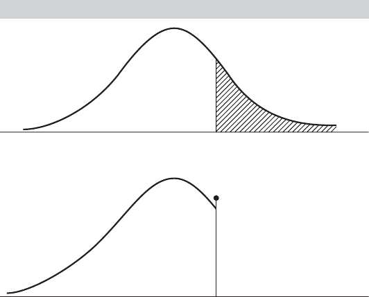
the untruncated population falls in the range that interests us. When data are censored,

the distribution that applies to the sample data is a mixture of discrete and continuous

distributions. Figure 19.4 illustrates the effects.

To analyze this distribution, we deﬁne a new random variable y transformed from

the original one, y

∗

,by

y = 0ify

∗

≤ 0,

y = y

∗

if y

∗

> 0.

FIGURE 19.4

Partially Censored Distribution.

Capacity Seats demanded

Capacity Tickets sold

CHAPTER 19

✦

Limited Dependent Variables

847

The distribution that applies if y

∗

∼ N[μ, σ

] is Prob(y = 0) = Prob(y

∗

≤ 0) =

(−μ/σ ) = 1 −(μ/σ ), and if y

∗

> 0, then y has the density of y

∗

This distribution is a mixture of discrete and continuous parts. The total probability

is one, as required, but instead of scaling the second part, we simply assign the full

probability in the censored region to the censoring point, in this case, zero.

THEOREM 19.3

Moments of the Censored Normal Variable

If y

∗

∼ N[μ, σ

] and y = aify

∗

≤ a or else y = y

∗

, then

E [y] = a + (1 − )(μ + σ λ),

and

Var[y] = σ

(1 − )[(1 − δ) + (α − λ)

],

where

[(a − μ)/σ ] = (α) = Prob(y

∗

≤ a) = , λ = φ/(1 − ),

and

δ = λ

− λα.

Proof: For the mean,

E [y] = Prob(y = a) × E [y | y = a] + Prob(y > a) × E [y | y > a]

= Prob(y

∗

≤ a) × a + Prob(y

∗

> a) × E [y

∗

| y

∗

> a]

= a + (1 − )(μ + σλ)

using Theorem 19.2. For the variance, we use a counterpart to the decomposition

in (B-69), that is, Var[y] = E [conditional variance] + Var[conditional mean],

and Theorem 19.2.

For the special case of a = 0, the mean simpliﬁes to

E [y |a = 0] = (μ/σ )(μ + σλ), where λ =

φ(μ/σ )

(μ/σ )

For censoring of the upper part of the distribution instead of the lower, it is only neces-

sary to reverse the role of  and 1 −  and redeﬁne λ as in Theorem 19.2.

Example 19.4 Censored Random Variable

We are interested in the number of tickets demanded for events at a certain arena. Our only

measure is the number actually sold. Whenever an event sells out, however, we know that the

actual number demanded is larger than the number sold. The number of tickets demanded

is censored when it is transformed to obtain the number sold. Suppose that the arena in

question has 20,000 seats and, in a recent season, sold out 25 percent of the time. If the

average attendance, including sellouts, was 18,000, then what are the mean and standard

deviation of the demand for seats? According to Theorem 19.3, the 18,000 is an estimate of

E[sales] = 20,000( 1 − ) + [μ + σλ].

Because this is censoring from above, rather than below, λ =−φ ( α)/( α) . The argu-

ment of , φ, and λ is α = (20,000 − μ) /σ . If 25 percent of the events are sellouts, then

 = 0.75. Inverting the standard normal at 0.75 gives α = 0.675. In addition, if α = 0.675,

848

PART IV

✦

Cross Sections, Panel Data, and Microeconometrics

then −φ(0.675)/0.75 = λ =−0.424. This result provides two equations in μ and σ , (a)

18,000 = 0.25( 20,000) + 0.75(μ − 0.424σ ) and (b) 0.675σ = 20,000 − μ. The solutions are

σ = 2426 and μ = 18,362.

For comparison, suppose that we were told that the mean of 18,000 applies only to the

events that were not sold out and that, on average, the arena sells out 25 percent of the

time. Now our estimates would be obtained from the equations (a) 18,000 = μ −0.424σ and

(b) 0.675σ = 20,000 − μ. The solutions are σ = 1820 and μ = 18,772.

19.3.2 THE CENSORED REGRESSION (TOBIT) MODEL

The regression model based on the preceding discussion is referred to as the censored

regression model or the tobit model [in reference to Tobin (1958), where the model

was ﬁrst proposed]. The regression is obtained by making the mean in the preceding

correspond to a classical regression model. The general formulation is usually given in

terms of an index function,

∗

= x



β + ε

= 0ify

∗

≤ 0,

= y

∗

if y

∗

> 0.

There are potentially three conditional mean functions to consider, depending on the

purpose of the study. For the index variable, sometimes called the latent variable,

E [y

∗

]isx



β. If the data are always censored, however, then this result will usu-

ally not be useful. Consistent with Theorem 19.3, for an observation randomly drawn

from the population, which may or may not be censored,

E [y

] = 









β + σλ

where

φ[(0 − x



β)/σ ]

1 − [(0 − x



β)/σ ]

φ(x



β/σ )

(x



β/σ )

. (19-12)

Finally, if we intend to conﬁne our attention to uncensored observations, then the re-

sults for the truncated regression model apply. The limit observations should not be

discarded, however, because the truncated regression model is no more amenable to

least squares than the censored data model. It is an unresolved question which of these

functions should be used for computing predicted values from this model. Intuition

suggests that E [y

] is correct, but authors differ on this point. For the setting in

Example 19.4, for predicting the number of tickets sold, say, to plan for an upcoming

event, the censored mean is obviously the relevant quantity. On the other hand, if the

objective is to study the need for a new facility, then the mean of the latent variable y

∗

would be more interesting.

There are differences in the partial effects as well. For the index variable,

∂E [y

∗

]

∂x

= β.

But this result is not what will usually be of interest, because y

∗

is unobserved. For the

observed data, y

, the following general result will be useful:

See Greene (1999) for the general result and Rosett and Nelson (1975) and Nakamura and Nakamura

(1983) for applications based on the normal distribution.