Gubbins D., Herrero-Bervera E. Encyclopedia of Geomagnetism and Paleomagnetism

Подождите немного. Документ загружается.

Malkus, W.V.R., and Proctor, M.R.E., 1974. The macrodynamics of

a-effect dynamos in rotating fluids. Journal of Fluid Mechanics,

67: 417–443.

Merrill, R.T., McElhinny, M.W., and McFadden, P.L., 1996. The

Magnetic Field of the Earth. San Diego, CA: Academic Press.

Moffatt, H.K., 1978. Magnetic Field Generation in Electrically

Conducting Fluids. Cambridge: Cambridge University Press.

Parker, E.N., 1955. The formation of sunspots from the solar toroidal

field. Astrophysics Journal, 121: 491–507.

Roberts, P.H., 1967. An Introduction to Magnetohydrodynamics.

London: Longmans.

Roberts, P.H., 1968. On the thermal instability of a rotating fluid

sphere containing heat sources. Philosophical Transactions of the

Royal Society of London A, 263:93–117.

Roberts, P.H., 1972. Kinematic dynamo models. Philosophical Trans-

actions of the Royal Society of London A, 272: 663–703.

Roberts, P.H., and Glatzmaier, G.A., 2000. A test of the frozen flux

approximation using geodynamo simulations. Philosophical Trans-

actions of the Royal Society of London A, 358: 1109–1121.

Roberts, P.H, Jones, C.A., and Calderwood, A., 2003. Energy

fluxes and ohmic dissipation. In Jones, C.A., Soward, A.M., and

Zhang, K. (eds.) Earth’s Core and Lower Mantle. London:

Taylor & Francis, pp. 100–129.

Rotvig, J., and Jones, C.A., 2002. Rotating convection-driven dyna-

mos at low Ekman number. Physical Review E, 66: 056308-1-15.

Sarson, G.R., 2000. Reversal models from dynamo calculations. Philo-

sophical Transactions of the Royal Society of London A, 358:

921–942.

Sarson, G.R., 2003. Kinematic dynamos driven by thermal-wind

flows. Proceedings of the Royal Society of London A, 459:

1241–1259.

Sarson, G.R., and Jones, C.A., 1999. A convection driven geodynamo

reversal model. Physics of the Earth and Planetary Interiors, 111:

3–20.

Schubert, G., Turcotte, D.L., and Olson, P., 2001. Mantle Convec-

tion in the Earth and Planets. Cambridge: Cambridge University

Press.

Sleep, N.H., 1990. Hot spots and mantle plumes: some phenomenol-

ogy. Journal of Geophysical Research, 95: 6715–6736.

Soward, A.M., and Jones, C.A., 1983. a

-dynamos and Taylor’s con-

straint. Geophysical and Astrophysical Fluid Dynamics, 27:

87–122.

Starchenko, S., and Jones, C.A., 2002. Typical velocities and magnetic

field strengths in planetary interiors. Icarus, 157: 426–435.

Steenbeck, M., Krause, F., and Rädler, K-H., 1966. A calculation of

the mean electromotive force in an electrically conducting fluid

in turbulent motion, under the influence of Coriolis forces. Zeits-

chrift für Naturforschung, 21a: 369–376.

Stevenson, D.J., 1982. Interiors of the giant planets. Annual Review of

Earth and Planetary Sciences, 10: 257–295.

Stevenson, D.J., 1987. Mercury magnetic field—a thermoelectric

dynamo. Earth and Planetary Science Letters, 82:114–120.

Stevenson, D.J., 2003. Planetary magnetic fields. Earth and Planetary

Science Letters, 208:1–11.

Taylor, J.B., 1963. The magneto-hydrodynamics of a rotating fluid and

the Earth’s dynamo problem. Proceedings of the Royal Society of

London A, 274: 274–283.

Tilgner, A., 2005. Precession driven dynamos. Physics of Fluids, 17:

034104-1.

Verhoogen, J., 1961. Heat balance in the Earth’s core. Geophysical

Journal, 4: 276–281.

Cross-references

Alfvén Waves

Antidynamo and Bounding Theorems

Boussinesq and Anelastic Approximations

Bullard, Edward Crisp (1907–1980)

Compass

Convection, Chemical

Convection, Nonmagnetic Rotating

Core Composition

Core Convection

Core Density

Core Magnetic Instabilities

Core Motions

Core Properties, Physical

Core Temperature

Core Turbulence

Core Viscosity

Core, Adiabatic Gradient

Core, Boundary Layers

Core, Electrical Conductivity

Core, Thermal Conduction

Core-based Inversions for the Main Geomagnetic Field

Core-Mantle Boundary, Heat Flow Across

Cowling’s Theorem

Crustal Magnetic Field

Depth to the Curie Temperature

Dynamo Waves

Dynamo, Model-Z

Dynamo, Solar

Dynamos, Experimental

Dynamos, Mean Field

Dynamos, Planetary and Satellite

Elsasser, Walter M. (1904–1991)

Fluid Dynamics Experiments

Gauss, Carl Friedrich (1777–1855)

Gellibrand, Henry (1597–1636)

Geodynamo, Energy Sources

Geodynamo, Numerical Simulations

Geomagnetic Jerks

Geomagnetic Secular Variation

Gilbert William (1544–1603)

Gravito-inertio Waves and Inertial Oscillations

Grüneisen’s Parameter for Iron and Earth’s Core

Halley, Edmond (1656–1742)

Harmonics, Spherical

Inhomogeneous Boundary Conditions and the Dynamo

Inner Core Composition

Inner Core Rotation

Inner Core Tangent Cylinder

Interiors of Planets and Satellites

Ionosphere

Larmor, Joseph (1857–1942)

Length of Day Variations, Decadal

Magnetic Field of Sun

Magnetoconvection

Magnetohydrodynamic Waves

Magnetohydrodynamics

Melting Temperature of Iron in the Core

Nondynamo Theories

Oscillations, Torsional

Precession and Core Dynamics

Proudman-Taylor Theorem

Radioactive Isotopes and their Decay in Core and Mantle

Reversals, Theory

Storms and Substorms, Magnetic

Taylor’s Condition

Thermal Wind

Verhoogen, John (1912–1993)

Westward Drift

296 GEODYNAMO

GEODYNAMO, DIMENSIONAL ANALYSIS AND

TIMESCALES

It is common to put the equations governing a complex physical sys-

tem like the geodynamo into dimensionless form. This clarifies the

importance of each term in the equations and can reduce the number

of input parameters to a minimum. Consider the very simple example

of the kinematic dynamo (q.v.), which is governed by a single partial

differential equation, the induction equation:

] B

¼rðv  B Þþ

B: (Eq. 1)

The fluid velocity is specified within a sphere and the induction

equation solved for a growing magnetic field. It depends on just three

input parameters: the amplitude of the velocity V, the radius of

the sphere c , and the electrical conductivity s. In dimensionless form

this reduces to just one input parameter, the magnetic Reynolds num-

ber R

¼ m

s Vc, where m

is the permeability of free space (see Tables

G2 and G3). Kinem atic dynamo behavior therefore depends on the

product of the three dimensional input parameter but not on all three

independently. This is a great help in exploring the behavior of the sys-

tem as a function of the input parameters. Incidentally, it means that

scaling the Earth down to a laboratory-sized experiment would require

a great increase in fluid velocity to compensate for the reduction in

length scale (increasing the conductivity is impossible since there are

no materials at room temperature with electrical conductivity signifi-

cantly higher than that of iron in the core).

Nondimensionalization is by no means a unique process: there are

many ways in which to scale the dimensional variables, each giving

different versions of the same equations. Consider once again the kine-

matic dynamo problem. The usual approach is to scale length with the

radius c and time with the magnetic diffusion time, m

s c

. This leads

to the form

] B

] t

¼ R

rðv  B Þþr

B: (Eq. 2)

so that R

can be regarded as a dimensionless measure of the fluid

velocity. A second way to nondimensionalize the induction equation

is to scale time with the overturn, or advection, time c/ V, the time it

takes for fluid to cross the sphere. This leads to the form

] B

] t

¼rðv  B ÞþR

 1

B : (Eq. 3)

Now the inverse magnetic Reynolds number is a dimensionless mea-

sure of magnetic diffusion. At first sight, Eqs. (2) and (3) appear

to contradict each other; the difference arises from the definition of

time, t.

In this article, I shall consider the fairly general case of a geody-

namo driven by a combination of heat and compositional buoyancy,

governed by the equations of momentum, induction, heat, and mass

transfer. The full geodynamo problem is usually put into a nondimen-

sional form that leaves just four independent input parameters, the

Rayleigh number R

, Ekman number E, the Prandtl number P

, and

the magnetic Prandtl number P

. These are defined and estimated in

Table G3. Other nondimensional numbers are calculated from the solu-

tion of the equation, although they can also be independent input para-

meters for subproblems. Two examples are the magnetic Reynolds

number, which depends on the fluid velocity and is therefore calcu-

lated from the convective flow from the full dynamo problem but is

Table G2 Illustrative numerical values of core parameters used

Property Symbol Molecular Turbulent

Density r 10

kg m

 3

Gravity g 0 –10 m s

 2

Core radius c 3 484 km

Inner core radius r

1 215 km

Outer core depth d ¼ c  r

2 269 km

Angular velocity O 7 :272  10

 5

Kinematic viscosity n 10

 6

1

1 at room

temperature

Electrical

conductivity

s 5  10

 1

Thermal

conductivity

k 50 W m

1

 1

Specific heat C

700 J kg

 1

1

Magnetic

diffusivity

¼ðm

sÞ

 1

1 :6m

1

1: 6m

 1

Thermal diffusivity k ¼ k ð rC

 1

7  10

7

 1

1: 6m

 1

Molecular diffusion

constant

D 10

 6

1

1: 6m

 1

Thermal expansion a 5  10

6

 1

Typical core

velocity

V 10

 4

1

Typical magnetic

field

B 1mT

Adiabatic gradient T

0 :1K km

 1

Core heat flux Q 5TW

Temperature

gradient

0 :5K km

 1

Those above the line are measured directly; those below the line are inferr ed from

putative core composi tion, tem perature, and pressure T

is the excess tem perature gra-

dient over the adiabat T

, as defined in Eq. (4). Current dynamo models usuall y

assume some form of turbul ence that brings the small diffusivities of heat, momentum

(viscosi ty), and mass up to the larger value of the electrical diffusivity. For ill ustration

I have taken these values equal to 1.6 when calculating turbulent values in Tables G3

and G4 .

Table G3 Dimensionless numbers

Name Definition Molecular Turbulent

Rayleigh R

¼ g D r

= kn 10

7  10

Modified Rayleigh R

¼ R

E ¼ gDr

d=kO 10

8  10

Buoyancy R

¼ gDr

d 33

Ekman E ¼ n=Oc

15

9

Prandtl P

¼ n=k 1.4 1

Magnetic Prandtl P

¼ m

sn ¼ n= 6  10

7

Roberts P

¼ k= 4  10

7

Schmidt P

¼ n=D 11

Magnetic Schmidt P

¼ =D 1:6  10

Lewis P

¼ D=k 1.4 1

Magnetic Reynolds R

¼ m

sVc 200 200

Elsasser L ¼ B

s=rO 11

Rossby R

¼ V =2Oc 2  10

7

2  10

7

Nusselt Q=ð4pc

Þ 77

Thermal Peclet P

¼ Vc=k 5  10

200

Mass Peclet P

¼ Vc=D 3  10

200

Those above the line appear explicitly in formulations of the geodynamo equations; those

below are derived from solutions to the geodynamo problem; those in column 4 are for

nominal turbulent values of the diffusivities, k ¼ n ¼ D ¼  ¼ 1:6m

1

. Rayleigh

and buoyancy numbers are calculated for thermal convection by replacing Dr

with

aDT, where r

is the departure from the adiabaticdensitygradient, and DT is the tempera-

ture difference from the adiabat. Values for compositional convection are likely to be

higher. Q

is the heat conducted down the adiabat.

GEODYNAMO, DIMENSIONAL ANALYSIS AND TIMESCALES 297

the sole input parameter for the kinematic dynamo as already men-

tioned; and the Elsasser number (see below), which depends on the

magnetic field strength but is the main input parameter to the magne-

toconvection problem, in which a magnetic field is imposed rather

than being self-generated.

The nondimensional numbers represent ratios of terms appearing in

the governing equations: they are ratios of forces in the momentum

equation, of magnetic induction in the induction equation, of heat

transfer in the heat equation, and of mass transfer in the material diffu-

sion equation. Further physical insight may be obtained by expressing

them as ratios of timescales. The Earth’s magnetic field varies on an

enormous range of timescales, from less than a year for geomagnetic

jerks (q.v.) to a million years between reversals, and its age is compar-

able with that of the Earth. Timescales contained within the geody-

namo equations span an even wider spectrum, from a single day, the

timescale of the Coriolis force, to the molecular viscous and heat dif-

fusion times, which exceed the age of the Earth itself (Table G4). This

enormous disparity of timescales makes numerical simulation of the

geodynamo very difficult, more so than the range of length scales

involved, because the computer must resolve details on the shortest

timescale, then integrate the equations for sufficient time to demon-

strate dynamo generation in order to follow the evolution. The very

long viscous and thermal diffusion times are impossible to simulate

and are usually shortened by assumed turbulent enhancement of the

diffusivities (see Core turbulence), often by simply equalizing the dif-

fusivities to the largest, electrical, diffusivity.

A summary of relevant timescales is given in Table G4. Diffusion

times are quoted by the formula shown; true diffusion times in a

sphere for magnetic, viscous, thermal, and compositional diffusion

contain the factor p

to give the time taken for a dipole field to fall

by a factor of e. Geometrical factors and wavenumbers have been

omitted from the formulae for dimensionless numbers in Table G5.

The periods of MAC waves depend on the wavenumber and are

considerably shorter than the time quoted in the table. Each group of

nondimensional parameters is now discussed in turn.

Rayleigh, modified Rayleigh, buoyancy numbers—

buoyancy: dissipation

The Rayleigh number multiplies the buoyancy force in the dimension-

less equation of motion and as such measures the driving force of the

convective dynamo. This discussion is restricted to thermal convection

but the same remarks apply to compositional convection with concen-

tration replacing temperature, D replacing k, and a compositional

expansion coefficient replacing a. I do not discuss complications

involving both thermal and compositional buoyancy since there has

been very little discussion of it in the literature to date, and no direct

observations.

is a complicated combination of dimensional parameters and is

very difficult to estimate numerically. For free convection heated from

below, a critical value of the Rayleigh number must be exceeded

before convection starts. This is because motion is opposed by viscous

forces and heat, the source of the buoyancy, can dissipate away by

conduction. Consider the balance of buoyancy and viscous forces

for a rising, hot, light blob: raDTg ¼ rnV

. The blob falls with

terminal (Stokes) velocity when buoyancy equals viscous drag,

of order V

¼ agDTd

=n. The time to rise through the core is

¼ d= V

¼ n=aDTgd. Buoyancy is lost by diffusion of heat into

the surrounding fluid, restricting the power of the convection. The

Rayleigh number is the ratio of the thermal diffusion time t

¼ d

to the viscous buoyant rise time: R

¼ gaDTd

=kn. Vigor of convec-

tion is measured by the speed with which fluid rises compared to the

speed with which heat is lost by conduction.

There are two major difficulties with estimating R

in the core. First,

it is virtually impossible to estimate the temperature difference DT

driving the convection. The correct boundary condition for core

convection is constant heat flux imposed by the convecting and cool-

ing mantle. This gives the temperature gradient at the core surface,

from which we must subtract the adiabatic gradient, which would hold

in the absence of any convection:

4pc

 T

: (Eq. 4)

We could then take DT to be the product of the temperature gradient

and the outer core depth d. The problem is that Q is very uncertain

and T

poorly known. We do know, however, that the core must con-

vect in order to produce a dynamo, and that T

must exceed the adiabat

by enough to power the dynamo. Gubbins (2001) estimates R

in this

way to be about 1000 times the critical value for nonmagnetic convec-

tion. Jones (2000) gives an independent argument based on the speed

of the flow in the core and arrives at a similar value. The critical Ray-

leigh number depends strongly on both rotation, which increases it,

and magnetic field, which in combination with rotation decreases it;

in the core seems to be close to the critical value in the absence

of any magnetic field (Gubbins, 2001). The Rayleigh number for com-

positional convection could be much higher.

Studies of magnetoconvection have shown that, at high rotation

rates, the critical Rayleigh number varies as E

1

, prompting some

authors to use the modified Rayleigh number R

E. This takes account,

to some extent, the effect of rotation on the stability of convection. R

Table G5 Dimensionless numbers and their relationship with

timescales

Rayleigh t

Modified Rayleigh t

Buoyancy t=t

Ekman t=t

Prandtl t

Magnetic Prandtl t



Roberts t



Schmidt t

Magnetic Schmidt t



Lewis t

Magnetic Reynolds t



Elsasser t



MAC

Rossby t=t

Thermal Péclet t

Mass Péclet t

Table G4 Timescales for the Earth’s core, definition, and

numerical estimates in years

Time Definition Molecular Turbulent

Magnetic diffusion

(core)



¼ c

=p

25000 25000

Magnetic diffusion

(inner core)

¼ r

=p

3000

Thermal diffusion t

¼ c

=kp

6  10

25000

Viscous diffusion t

¼ c

=np

4  10

25000

Mass diffusion t

¼ c

=Dp

4  10

25000

Overturn t

¼ d=V 700

Buoyant rise t

¼ n=aDTgd 2  10

19

3  10

13

Coriolis rise t

¼ cO=gaDT 10

4

Day t 3  10

3

MAC wave t

MAC

¼ Orm

3  10

298 GEODYNAMO, DIMENSIONAL ANALYSIS AND TIMESCALES

contains only the thermal diffusivity and not the fluid viscosity, which

plays a negligible role in resisting the flow compared to the magnetic

force. The presumed force balance is between Coriolis and buoyancy

forces, leading to the scaling gaDT  OV; the relevant timescale

is then

¼ c=V ¼

gaDT

The modified Rayleigh number is then seen as the ratio of thermal

diffusion time to Coriolis rise time t

. Others have used a buoy-

ancy parameter that involve s no diffusivity. This is the ratio of the

day to the Coriolis rise time. Further details may be found in, for

example, Gubbins and Roberts (1987).

Nusselt number—convected heat: conducted heat

The Nusselt number is a different dimensionless measure of the heat

driving the convection. It is usually quoted as the ratio of convected

heat flux to conducted heat flux for convection between boundaries

with fixed temperatures. The situation in the Earth’s outer core is

somewhat different. First, the boundary conditions are fixed tempera-

ture at the bottom (melting temperature) and fixed heat flux at the

top (as dictated by mantle convection). The Nusselt number is there-

fore, in some sense, an input parameter for the geodynamo problem.

Second, the conduction profile includes the adiabatic gradient, which

is steep and responsible for conduction of a large amount of heat in

the context of the Earth’s thermal history. It is not really an estimate

of the vigor of the convection, which depends on the superadiabatic

temperature gradient rather than the absolute value. Estimates of N

in the core are inevitably restricted to low values, from 1 to 10,

because of limits on the heat coming from the core.

Ekman number—viscous force: Coriolis force

E is tiny, whether we use molecular or turbulent values of the viscos-

ity, reflecting the enormous disparity between the viscous and diurnal

timescales. Smallness of E causes the greatest difficulty in numerical

simulations of the geodynamo, even when turbulent diffusivities are

used. The smallest values of E achieved in numerical simulations so

far are 10

5

–10

7

, compared with E ¼ 10

9

for the Earth’s core

assuming a turbulent viscosity.

Rossby number—inertial: Coriolis force

is a measure of the importance of inertial forces Dv/Dt in the equa-

tion of motion. It is small in the core and many studies have dropped

the inertial terms altogether. This may not be appropriate, since inertial

terms may play a role in restoring the balance between magnetic,

buoyancy, and rotational forces. Inertia also plays an essential role in

torsional oscillations (q.v.).

Prandtl numbers

The Prandtl number measures the ratio of viscous to thermal diffusion.

Liquid metals generally have small Prandtl numbers of order 0.1, and

many studies have focused on this. Others have taken P

¼ 1, consis-

tent with the assumption of turbulence equalizing the diffusivities. P

and P

also have extremely low values that cause problems. Similar

remarks apply to compositional diffusion.

Magnetic Reynolds number—induction: magnetic

diffusion

is a dimensionless measure of the fluid velocity, the input para-

meter for kinematic dynamos, and is the ratio of the overturn and mag-

netic diffusion times. It must exceed a critical value for dynamo action,

for which there are lower bounds (see Antidynamo and bounding the-

orems). Estimates of fluid flow in the core, based on inferences from

secular variation, yields R

 200, low but well above the critical

values required for dynamo action.

clet numbers—advection: diffusion

Like the magnetic Reynolds numbers, P

and P

measure the impor-

tance of advection in the heat and mass transfer equations, respec-

tively. They are the ratios of the day to viscous diffusion time, and

day to compositional diffusion times, respectively.

Elsasser number—magnetic: Coriolis force

L is a dimensionless measure of the Lorentz force and an essential input

parameter for magnetoconvection. The balance between magnetic,

buoyancy, and Coriolis forces (MAC) leads to magnetohydrodynamic

waves with periods of centuries to millennia (see Magnetohydrody-

namic waves). They are highly dispersive and under certain simple con-

ditions have wavespeeds given by V

MAC

¼ kB

=Orm

, where k is the

wavenumber. A “MAC” timescale can then be defined as the time taken

for a MAC wave with wavelength c to cross the core,

MAC

Orm

The Elsasser number is then L ¼ t



MAC

. Small L is the condition

for large-scale MAC waves to pass through the core with little dissipa-

tion. The numerical value for t

MAC

in Table G4 is rather long: a typical

MAC wave with wavelength 1000 km would have timescale closer to

1 ka; a stronger core field of 10 mT, the value usually taken in MAC

wave studies, would reduce it by a factor of 100.

Less common dimensionless numbers

The above list includes those in common usage in geodynamo theory.

Other numbers are used occasionally, and some have different names.

The Taylor number is the inverse square of the Ekman number, the

ratio of centrifugal to viscous force (and for the core is one of the big-

gest numbers one is ever likely to come across!). The Chandrasekhar

number B

is a useful measure of the magnetic force in place

of the Elsasser number when rotation is unimportant; it measures the

relative strengths of magnetic and diffusive forces. The Hartmann

number, Bs

d=m

1=2

, is important in boundary layer theory; it mea-

sures the ratio of magnetic to viscous forces. The Alfvén (q.v.) number,

Vðrm

=B, is a magnetic Mach number, the ratio of flow speed to

the speed of Alfvén waves. Its inverse is the Cowling number. Neither

are in common use in geomagnetism, although Merrill and McElhinny

(1996) define the Alfvén number as the Cowling number. The degree

to which magnetic fields are frozen-in is usefully measured by the

Lundqvist number, m

sB=r

, the time for Alfvén waves to cross

the core divided by the magnetic diffusion time.

David Gubbins

Bibliography

Gubbins, D., 2001. The Rayleigh number for convection in the Earth’s

core. Physics of the Earth and Planetary Interiors, 128:3–12.

Gubbins, D., and Roberts, P.H., 1987. Magnetohydrodynamics of

the Earth’s core. In Jacobs, J.A. (ed.), Geomagnetism, Vol. II,

Chapter 1. London: Academic Press, pp. 1–183.

Jones, C.A., 2000. Convection-driven geodynamo models. Philosophi-

cal Transactions of the Royal Society of London, Series A, 873:

873–897.

Merrill, R.T., and McElhinny, M.W., 1996. The Magnetic Field of the

Earth. San Diego, CA: Academic Press.

GEODYNAMO, DIMENSIONAL ANALYSIS AND TIMESCALES 299

Cross-references

Alfvén, Hannes Olof Gösta (1908–1995)

Antidynamo and Bounding Theorems

Convection, Chemical

Convection, Nonmagnetic Rotating

Core, Adiabatic Gradient

Core Convection

Core Motions

Core Turbulence

Dynamos, Kinematic

Geodynamo

Geodynamo, Numerical Simulations

Geomagnetic Jerks

Geomagnetic Spectrum, Temporal

Magnetoconvection

Magnetohydrodynamic Waves

Magnetohydrodynamics

Oscillations, Torsional

GEODYNAMO, ENERGY SOURCES

The magnetic field of the Earth is maintained against ohmic losses by

dynamo action in the fluid core which takes its energy from several

sources of different natures and amplitudes, all being consequences

of the thermal evolution of the core. Moreover, each source has a dif-

ferent efficiency in maintaining ohmic dissipation compared to the

others. The study of these problems is then of major importance for

understanding dynamo theory as well as the thermal evolution of

the Earth.

Evolving reference state

The core of the Earth is composed of iron, nickel, and some lighter ele-

ments, with concentrations that are still matter of lively debates (see

Core composition, and Poirier, 1994). The light elements play a very

important dynamical role in maintaining the geodynamo since their

rejection upon inner core crystallization drives compositional convec-

tion in the core (see Convection, chemical). The core is therefore usually

modeled as a binary alloy of Fe and some light element X. Including a

more realistic chemistry in thermal evolution models on the core would

add complexity (although no real difficulty) in the derivations without

really improving the understanding, unless not yet documented coupled

effects occur.

The Earth’s core is different from a well-controlled convection

experiment in a laboratory, in the fact that it is continually evolving

on geological timescales and that the energy for the motion comes

from that evolution. Fortunately, the timescales relevant for this evolu-

tion and that for the dynamics are very different and can be separated.

To get expressions for the different energy sources in the balance, we

need to know in what state is the core when averaged on a timescale

long compared to the one relevant to the dynamics but short compared

to the one associated with the thermal evolution. The short-time

dynamics is responsible for maintaining the core close to that reference

state whereas the evolution of the reference state provides the energy

sources needed by the dynamics.

Convection in the liquid core is assumed to be very efficient so

that, outside of tiny boundary layers (see Core, boundary layers), all

extensive quantities responsible for the movement (entropy s and

mass fraction of light elements x) are uniform: rx ¼ 0 and rs ¼ 0.

In addition, the momentum equation is assumed to average to the

hydrostatic balance: rp ¼ rg, with r the density and g the accelera-

tion due to gravity. It is often useful to know what the temperature is

in the reference state (see Core temperature) and isentropy and iso-

chemistry implies it to be adiabatic (see Core, adiabatic gradient)

rT ¼ agT=C

, with a the coefficient of thermal expansion and C

the heat capacity at constant pressure.

The set of partial differential equations defining the reference state

must be supplemented by an equation of state relating the density to

the pressure, for example at constant entropy, and by boundary condi-

tions. In terms of temperature, the equilibrium between solid and liquid

at the inner core boundary (ICB) provides the required condition, the

liquidus of the core alloy being given (see Melting temperature of iron

in the core, Theory and melting temperature of iron in the core, experi-

mental) as a function of radius in the core. Depending on the choice of

equation of state, one can get different expressions for the different

profiles in the reference state, usually in the form of some series

expansion of powers of the radius.

It should be noted that the actual averaged state cannot be exactly

hydrostatic, owing to its being compressible and compressing with

time, but the corrections to this balance are negligible for the ener-

getics of the core (Braginsky and Roberts, 1995). The deviations from

the isentropic, well mixed state can also be estimated from the ampli-

tude of fluid velocity at the top of the core which also allows an

estimate of the typical scale for the size of boundary layers. These

are found to be a negligible contribution to averaged quantities (e.g.,

Braginsky and Roberts, 1995), although they are very important for

the dynamics of the core.

Energy equation

The equation for total (internal, kinetic, magnetic, and gravitational)

energy conservation can be integrated over the volume of the core

and it states that the total heat loss of the core, the heat flow across

the core-mantle boundary (CMB), is balanced by the sum of four

terms, the secular cooling Q

associated with the heat capacity

of the core, the latent heat Q

associated with the gradual freezing of

the inner core, the gravitational energy E

associated with the rearran-

gement in the outer core of the light elements that are released at the

ICB by the freezing of the inner core, and possibly the radioactive

heating Q

CMB

¼ Q

þ Q

þ E

þ Q

: (Eq. 1)

The first three terms are related to the growth of the inner core and can

be written as a function of the radius of the inner core c times its time

derivative. The exact expression of these three functions depends on

the choice of equation of state and parameterization and the expres-

sions of Labrosse (2003) can be written to first order as:

ðcÞ 1 



; (Eq. 2)

¼ 4pc

rðcÞT

ðcÞDS

; (Eq. 3)

GDrr





; (Eq. 4)

with b and c the radii of the outer and inner core respectively, r

the

central density, C

the heat capacity, T

the liquidus temperature, g

the Grüneisen parameter (see Grüneisen’s parameter for iron and

Earth’s core), L

the adiabatic length scale, DS the entropy of crystal-

lization, Dr the chemical density jump across the ICB (see Core den-

sity), and G the gravitational constant. All these physical parameters

can be estimated with more or less accuracy using combinations of

geophysical data (mostly seismology) and mineral physics (see Core

properties, physical; Core properties, theoretical determination).

Convective mixing can be assumed to be sufficient to ensure a

uniform mass rate hðtÞ of radioactive heating in the core. Therefore,

300 GEODYNAMO, ENERGY SOURCES

radioactive heating is not related to inner core growth and is simply

equal to M

h ðt Þ , with M

the mass of the core. This energy source

can then be easily computed, provided one knows the concentration

in radioactive elements in the core. Among all possible heat producing

isotopes,

K has always been the most popular candidate, owing to its

apparent depletion in the mantle compared to Earth forming meteorites

and its predicted metalization at high pressure that would allow it to

enter the core. However, potassium is also somewhat volatile and its

budget in the Earth is influenced by accretion processes. In addition,

the concentration of potassium in the core depends strongly on the sce-

nario of core formation, a process still far from perfectly understood

(e.g., Stevenson, 1990). The most recent experiments devoted to the

partitioning of potassium between iron and silicates (e.g., Gessmann

and Wood, 2002; Lee and Jeanloz, 2003; Rama Murthy et al., 2003)

favor a concentration of potassium in the core of O(100) ppm, produ-

cing less than 1 TW at present but exponentially more in the past. Such

a value is too small to affect importantly the thermal evolution of the

core (Labrosse, 2003) and radioactivity will not be considered further.

The gravitational energy actually comes in the equations as a

compositional energy, due to a change of composition in a gradient

of chemical potential (Braginsky and Roberts, 1995; Lister and

Buffett, 1995). It is equal to the change of gravitational energy due

only to chemical stratification of the core. Other sources of change

of gravitational energy do not contribute significantly to this balance

and are mostly stored as strain energy.

As can be seen on Eqs. (2 – 4), for the different energy sources to be

estimated, one needs to know the growth rate of the inner core. Since

there is no direct way of measuring this number, one usually uses an

estimate of the heat flow across the CMB to get this number from the

energy balance (1). The heat flow across the CMB is not very well-known

(see Core-mantle boundary, heat flow across) but for a value of 10 TW

(say) and no radioactive elements, one gets approximately (Labrosse,

2003) Q

¼ 5 :5TW; Q

¼ 2 : 8TW; E

¼ 1 :7 TW.

The energy balance can be used for any time in the history of the Earth

to give the growth history of the inner core and the evolution of all

energy sources in the balance, provided the heat flow across the CMB

is known as a function of time. Moreover, this equation can be

integrated between the onset time of inner core crystallization and

the present to compute the age of the inner core (Labrosse et al .,

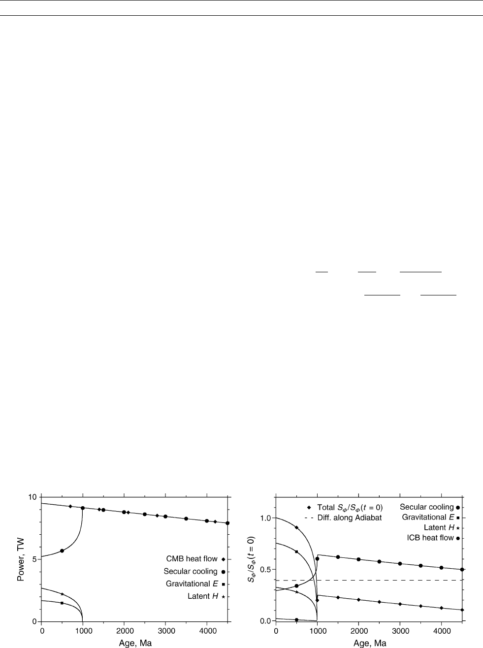
2001). A typical example of time evolution of the energy balance

is shown on Figure G12 , where the onset of inner core crystalliza-

tion, at an age of 1 Ga, is marked by a qualitative change in the

balance: before, only secular cooling is balancing Q

CMB

(in absence

of radioactivity) but this term is greatly decreased when the inner

core starts to crystallize and both latent heat and compositional

energy come in the balance.

En tropy equatio n

The energy equation does not involve the magnetic field directly and

contains no contribution from the dissipative heating. This is a well-

known characteristic of convective engines: in contrary to Carnot

engines, dissipation occurs inside the system and is then not lost. In

order to relate the energy sources to the magnetic field generation,

an entropy balance equation must be written. This equation comes

from a combination of the momentum balance equation and the energy

balance equation written above (e.g., Braginsky and Roberts, 1995)

and states that the entropy that flows out through the CMB is balanced

by the sum of the entropy that flows in due to the different heat

sources and the entropy that is produced by nonreversible processes,

mostly ohmic dissipation and conduction along the adiabatic tempera-

ture profile. This equation does not directly involve the gravitational

energy, since it is not a heat source. It can however, be brought back

into the equation by use of the energy balance to suppress the heat

flow across the CMB, giving an efficiency equation,

F þT



dV ¼

CMB

ICB

T

CMB

ICB

ðQ

ICB

þQ



T

CMB

T

CMB



;

(Eq. 5)

where it can be seen that each energy source contributes in maintaining

both the total ohmic dissipation F and the conduction along the adia-

batic gradient, but with different efficiency factors. In particular, this

equation shows that the gravitational energy has an efficiency factor

that is the ratio of the effective temperature T

at which ohmic dissipa-

tion occurs to the temperature at the CMB, T

CMB

, whereas all heat

sources efficiency factors have a contribution from the classical Carnot

engine efficiency factor, ðT

 T

CMB

Þ=T

, with T

the temperature at

which the heat source X is provided. This shows that compositional

energy is more efficiently transformed in dissipation than all heat

sources and that the efficiency of each heat source depends on the

temperature at which it is provided.

Figure G12 Energy (left) and entropy (right) balances of the core as a function of time for a typical evolution model without

radioactivity. (After Labrosse, 2003).

GEODYNAMO, ENERGY SOURCES 301

The energy sources on the right-hand side of Eq. (5) are the same as

that appearing in the energy balance Eq. (1) and, except for T

, their

efficiency factors can be expressed using the parameters characterizing

the reference state of the core. It can then be proved that all terms, except

the radioactive heating one, is a function of the radius of the inner core

and is proportional to its growth rate. This means that, if the heat flow

across the CMB is known, this growth rate can be computed from the

energy equation (1), and the entropy equation (5) then gives the ohmic

dissipation that is maintained. Alternatively, one can take the opposite

view and compute the growth rate of the inner core that is required to

maintain a given ohmic dissipation, the energy balance being then

used to get the heat flow across the CMB that makes this growth rate

happen. Unfortunately, the ohmic dissipation in the core is no better

known than the heat flow across the CMB, since it is dominated by

small-scales of the magnetic field and possibly by the invisible toroidal

part of it (Gubbins and Roberts, 1987; Roberts et al., 2003). However,

the value of Q

CMB

¼ 10 TW used above gives a contribution of ohmic

dissipation to the entropy balance F=T

¼ 500 MWK

1

. The tem-

perature T

is not well-known, but is bounded by the temperature at

the inner core boundary and the CMB and this gives F ’ 2 TW.

The evolution with time of the entropy balance associated with a

given heat flow evolution can be computed and the example shown

above gives the result of Figure G12. An interesting feature is the

sharp increase of the ohmic dissipation in the core when the inner core

starts crystallizing, latent heat and, even more so, gravitational energy

being more efficient than secular cooling. Unfortunately, the link

between this ohmic dissipation and the magnetic field observed at

the surface of the Earth is far from obvious and the detection of such

an increase in the paleomagnetic record is unlikely (Labrosse and

Macouin, 2003).

Some alternative models for the average structure of the core invol-

ving some stratification have been proposed. In particular, the heat

conducted along the adiabatic temperature gradient can be rather large

(about 7 TW) and might be larger than the heat flow across the CMB

(see Core-mantle boundary, heat flow across). In this case, two differ-

ent models have been proposed. In the first one, the adiabatic tempera-

ture profile is maintained by compositional convection against thermal

stratification, except in a still very thin boundary layer, and this means

that the entropy flow across the CMB is less than that required to

maintain the conduction along the average temperature profile. In

other words, the compositional convection has to fight against thermal

stratification to maintain the adiabatic temperature profile in addition

to maintaining the dynamo. In the second model (see Labrosse et al.,

(1997); Lister and Buffett (1998)), a subadiabatic layer of several hun-

dreds of kilometers is allowed to develop at the top of the core and the

entropy flow out of the core balances the conduction along the average

temperature gradient. In this case, the compositional energy is entirely

used for the dynamo. Which of these two options would be chosen by

the core is a dynamical question that cannot be addressed by simple

thermodynamic arguments as used here.

Stéphane Labrosse

Bibliography

Braginsky, S.I., and Roberts, P.H., 1995. Equations governing convec-

tion in Earth’s core and the geodynamo. Geophysical Astrophysical

Fluid Dynamics, 79:1–97.

Gessmann, C.K., and Wood, B.J., 2002. Potassium in the Earth’s core?

Earth and Planetary Science Letters, 200:63–78.

Gubbins, D., and Roberts, P.H., 1987. Magnetohydrodynamics of the

Earth’s core. In Jacobs, J.A., (ed.), Geomagnetism, Vol. 2. London:

Academic Press, pp. 1–183.

Labrosse, S., 2003. Thermal and magnetic evolution of the Earth’s

core. Physics of the Earth and Planetary Interiors, 140: 127– 143.

Labrosse, S., and Macouin, M., 2003. The inner core and the geody-

namo. Comptes Rendus Geosciences, 335:37–50.

Labrosse, S., Poirier, J.-P., and Le Mouël, J.-L., 1997. On cooling of

the Earth’s core. Physics of the Earth and Planetary Interiors,

99:1–17.

Labrosse, S., Poirier, J.-P., and Le Mouël, J.-L., 2001. The age of the

inner core. Earth and Planetary Science Letters, 190:111–123.

Lee, K.K.M., and Jeanloz, R., 2003. High-pressure alloying of potas-

sium and iron: radioactivity in the Earth’s core? Geophysical

Research Letters, 30: 2212, doi:10.1029/2003GL018515.

Lister, J.R., and Buffett, B.A., 1995. The strength and efficiency of the

thermal and compositional convection in the geodynamo . Physics

of the Earth and Planetary Interiors, 91:17–30.

Lister, J.R., and Buffett, B.A., 1998. Stratification of the outer core at

the core-mantle boundary. Physics of the Earth and Planetary

Interiors, 105:5–19.

Poirier, J.-P., 1994. Light elements in the Earth’s core: a critical

review. Physics of the Earth and Planetary Interiors, 85: 319–

337.

Rama Murthy, V., van Westrenen, W., and Fei, Y., 2003. Radioactive

heat sources in planetary cores: experimental evidence for potas-

sium. Nature, 423: 163–165.

Roberts, P.H., Jones, C.A., and Calderwood, A.R., 2003. Energy

fluxes and ohmic dissipation in the Earth’s core. In Jones, C A.,

Soward, A.M., and Zhang, K. (eds.) Earth’s Core and Lower Man-

tle. London: Taylor & Francis, pp. 100–129.

Stevenson, D.J., 1990. Fluid dynamics of core formation. In Newsom,

H.E., and Jones, J.H. (eds.) Origin of the Earth. New York: Oxford

University Press, pp. 231–249.

Cross-references

Convection, Chemical

Core Composition

Core Density

Core Properties, Physical

Core Properties, Theoretical Determination

Core Temperature

Core, Adiabatic Gradient

Core, Boundary Layers

Core-Mantle Boundary, Heat Flow Across

Grüneisen’s Parameter for Iron and Earth’s Core

Melting Temperature of Iron in the Core, Experimental

Melting Temperature of Iron in the Core, Theory

GEODYNAMO: NUMERICAL SIMULATIONS

Introduction

The geodynamo is the name given to the mechanism in the Earth’s

core that maintains the Earth’s magnetic field (see Geodynamo). The

current consensus is that flow of the liquid iron alloy within the outer

core, driven by buoyancy forces and influenced by the Earth’s rota-

tion, generates large electric currents that induce magnetic field, com-

pensating for the natural decay of the field. The details of how this

produces a slowly changing magnetic field that is mainly dipolar in struc-

ture at the Earth’s surface, with occasional dipole reversals, has been the

subject of considerable research by many people for many years.

The fundamental theory, put forward in the 1950s, is that differential

rotation within the fluid core shears poloidal (north-south and radial)

magnetic field lines into toroidal (east-west) magnetic field; and

three-dimensional (3D) helical fluid flow twists toroidal field lines into

poloidal field. The more sheared and twisted the field structure the

faster it decays away; that is, magnetic diffusion (reconnection) conti-

nually smooths out the field. The field is self-sustaining if, on average,

the generation of field is balanced by its decay. Discovering and under-

standing the details of how rotating convection in Earth’s fluid outer

302 GEODYNAMO: NUMERICAL SIMULATIONS

core maintains the observed intensity, structure, and time dependencies

requires 3D computer models of the geodynamo.

Magnetohydrodynamic (MHD) dynamo simulations are numerical

solutions of a coupled set of nonlinear differential equations that

describe the 3D evolution of the thermodynamic variables, the fluid

velocity, and the magnetic field. Because so little can be detected about

the geodynamo, other than the poloidal magnetic field at the surface

(today’s field in detail and the paleomagnetic field in much less detail)

and what can be inferred from seismic measurements and variations

in the length of the day and possibly in the gravitational field, models

of the geodynamo are used as much to predict what has not been

observed as they are used to explain what has. When such a model

generates a magnetic field that, at the model’s surface, looks qualita-

tively similar to the Earth’s surface field in terms of structure, inten-

sity, and time-dependence, then it is plausible that the 3D flows and

fields inside the model core are qualitatively similar to those in the

Earth’s core. Analyzing this detailed simulated data provides a physi-

cal description and explanation of the model’s dynamo mechanism

and, by assumption, of the geodynamo.

The first 3D global convective dynamo simulations were developed

in the 1980s to study the solar dynamo. Gilman and Miller (1981) pio-

neered this style of research by constructing the first 3D MHD dynamo

model. However, they simplified the problem by specifying a constant

background density, i.e., they used the Boussinesq approximation of

the equations of motion. Glatzmaier (1984) developed a 3D MHD

dynamo model using the anelastic approximation, which accounts for

the stratification of density within the sun. Zhang and Busse (1988) used

a 3D model to study the onset of dynamo action within the Boussinesq

approximation. However, the first MHD models of the Earth’s dynamo

that successfully produced a time-dependent and dominantly dipolar

field at the model’s surface were not published until 1995 (Glatzmaier

and Roberts, 1995; Jones et al., 1995; Kageyama et al., 1995). Since

then, several groups around the world have developed dynamo models

and several others are currently being designed. Some features of the

various simulated fields are robust, like the dominance of the dipolar part

of the field outside the core. Other features, like the 3D structure and

time-dependence of the temperature, flow, and field inside the core,

depend on the chosen boundary conditions, parameter space, and numer-

ical resolution. Many review articles have been written that describe and

compare these models (e.g., Hollerbach, 1996; Glatzmaier and Roberts,

1997; Fearn, 1998; Busse, 2000; Dormy et al., 2000; Roberts and

Glatzmaier, 2000; Christensen et al., 2001; Busse, 2002; Glatzmaier,

2002; Kono and Roberts, 2002).

Model description

Models are based on equations that describe fluid dynamics and mag-

netic field generation. The equation of mass conservation is used with

the very good assumption that the fluid flow velocity in the Earth’s outer

core is small relative to the local sound speed. The anelastic version of

mass conservation accounts for a depth-dependent background density;

the density at the bottom of the Earth’s fluid core is about 20% greater

than that at the top. The Boussinesq approximation simplifies the equa-

tions further by neglecting this density stratification, i.e., by assuming a

constant background density. An equation of state relates perturbations

in temperature and pressure to density perturbations, which are used

to compute the buoyancy forces, which drive convection. Newton’s

second law of motion (conservation of momentum) determines how

the local fluid velocity changes with time due to buoyancy, pressure

gradient, viscous, rotational (Coriolis), and magnetic (Lorentz) forces.

The MHD equations (i.e., Maxwell’s equations and Ohm’s law with

the extremely good assumption that the fluid velocity is small relative

to the speed of light) describe how the local magnetic field changes with

time due to induction by the flow and diffusion due to finite conductiv-

ity. The second law of thermodynamics dictates how thermal diffusion

and Joule and viscous heating determine the local time rate of change

of entropy (or temperature). Additional equations are sometimes

included that account for perturbations in composition and gravitational

potential and their effects on buoyancy.

This set of coupled nonlinear differential equations, with a set

of prescribed boundary conditions, is solved each numerical time step

to obtain the evolution in 3D of the fluid flow, magnetic field,

and thermodynamic perturbations. Most geodynamo models have

employed spherical harmonic expansions in the horizontal directions

and either Chebyshev polynomial expansions or finite differences in

radius. The equations are integrated in time typically by treating the

linear terms implicitly and the nonlinear terms explicitly. The review

articles mentioned above describe the variations on the equations,

boundary conditions, and numerical methods employed in the various

models of the geodynamo.

Current results

Since the mid-1990s, 3D computer simulations have advanced our

understanding of the geodynamo. The simulations show that a domi-

nantly dipolar magnetic field, not unlike the Earth’s, can be maintained

by convection driven by an Earth-like heat flux. A typical snapshot of

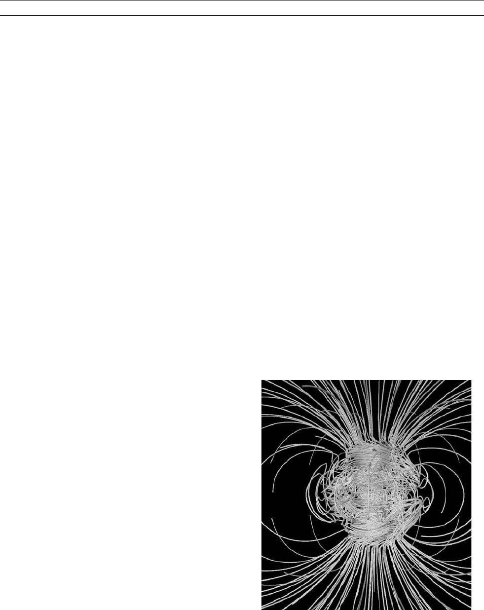
the simulated magnetic field from a geodynamo model is illustrated in

Figure G13 with a set of field lines. In the fluid outer core, where the

field is generated, field lines are twisted and sheared by the flow. The

field that extends beyond the core is significantly weaker and domi-

nantly dipolar at the model’s surface, not unlike the geomagnetic field.

For most geodynamo simulations, the nondipolar part of the surface

field, at certain locations and times, propagates westward at about

0.2



1

as has been observed in the geomagnetic field over the past

couple hundred years.

Several dynamo models have electrically conducting inner cores

that on average drift eastward relative to the mantle (e.g., Glatzmaier

and Roberts, 1995; Sakuraba and Kono, 1999; Christensen et al.,

2001), opposite to the propagation direction of the surface magnetic

Figure G13 A snapshot of the 3D magnetic field simulated with

the Glatzmaier-Roberts geodynamo model and illustrated with a

set of magnetic field lines. The axis of rotation is vertical and

centered in the image. The field is complicated and intense

inside the fluid core where it is generated by the flow; outside the

core it is a smooth, dipole-dominated, potential field. (From

Glatzmaier, 2002.)

GEODYNAMO: NUMERICAL SIMULATIONS 303

field. Inside the fluid core the simulated flow has a “thermal wind”

component that, near the inner core, is predominantly eastward relative

to the mantle. Magnetic field in these models that permeates both this

flow and the inner core tries to drag the inner core in the direction of

the flow. This magnetic torque is resisted by a gravitational torque

between the mantle and the topography on the inner core surface.

The amplitude of the superrotation rate predicted by geodynamo mod-

els depends on the model’s prescribed parameters and assumptions and

on the very poorly constrained viscosity assumed for the inner core’s

deformable surface layer, which by definition, is near the melting

temperature. The original prediction was an average of about 2



long-

itude per year faster than the surface. Since then, the superrotation rate

of the Earth’s inner core (today) has been inferred from several seismic

analyses, but is still controversial. There is a spread in the inferred

values, from the initial estimates of 1



to 3



eastward per year (relative

to the Earth’s surface) to some that are zero to within an uncertainty of

0.2



per year. More recent geodynamo models that include an inhibit-

ing gravitational torque also predict smaller superrotation rates.

On a much longer timescale, the dipolar part of the Earth’s field

occasionally reverses (see Reversals, theory). The reversals seen in

the paleomagnetic record are nonperiodic. The times between reversals

are measured in hundreds of thousands of years; whereas the time to

complete a reversal is typically a few thousand years, less than a mag-

netic dipole decay time. Several dynamo simulations have produced

spontaneous nonperiodic magnetic dipole reversals (Glatzmaier and

Roberts, 1995; Glatzmaier et al., 1999; Kageyama et al., 1999; Sarson

and Jones, 1999; Kutzner and Christensen, 2002). Regular (periodic)

reversals, like the dynamo-wave (q.v.) reversals seen in early solar

dynamo simulations, have also occurred in recent dynamo simulations.

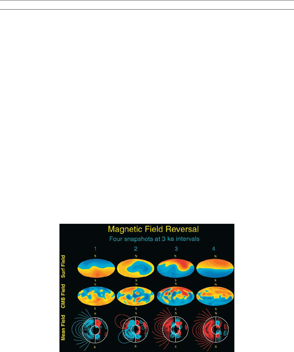
One of the simulated reversals is portrayed in Figure G14/Plate 16

with four snapshots spanning about 9 ka. The radial component of

the field is shown at both the core-mantle boundary (CMB) and the

surface of the model Earth. The reversal, as viewed in these surfaces,

begins with reversed magnetic flux patches in both the northern and

southern hemispheres. The longitudinally averaged poloidal and

toroidal parts of the field inside the core are also illustrated at these

times. Although when viewed at the model’s surface, the reversal

appears complete by the third snapshot, another 3 ka is required for

the original field polarity to decay out of the inner core and the new

polarity to diffuse in.

Small changes in the local flow structure continually occur in this

highly nonlinear chaotic system. These can generate local magnetic

anomalies that are reversed relative to the direction of the global dipo-

lar field structure. If the thermal and compositional perturbations con-

tinue to drive the fluid flow in a way that amplifies this reversed field

polarity while destroying the original polarity, the entire global field

structure would eventually reverse. However, more often, the local

reversed polarity is not able to survive and the original polarity fully

recovers because it takes a couple of thousand years for the original

polarity to decay out of the solid inner core. This is a plausible expla-

nation for “events,” which occur when the paleomagnetic field (as

measured at the Earth’s surface) reverses and then reverses back, all

within about 10 ka.

On an even longer timescale, the frequency of reversals seen in the

paleomagnetic record varies. The frequency of nonperiodic reversals in

geodynamo simulations has been found to depend on the pattern of

outward heat flux imposed over the CMB (presumably controlled in

the Earth by mantle convection) and on the magnitude of the convec-

tive driving relative to the effect of rotation.

Many studies have been conducted via dynamo simulations to,

for example, assess the effects of the size and conductivity of the

solid inner core, of a stably stratified layer at the top of the core, of

Figure G14/Plate 16 A sequence of snapshots of the longitudinally averaged magnetic field through the interior of the core and of the

radial component of the field at the core-mantle boundary and at what would be the surface of the Earth, displayed at roughly 3 ka

intervals spanning a dipole reversal from a geodynamo simulation. In the plots of the average field, the small circle represents the inner

core boundary and the large circle is the core-mantle boundary. The poloidal field is shown as magnetic field lines on the left-hand

sides of these plots (blue is clockwise and red is counterclockwise). The toroidal field direction and intensity are represented as

contours (not magnetic field lines) on the right-hand sides (red is eastward and blue is westward). Aitoff-Hammer projections of the

entire core-mantle boundary and surface are used to display the radial component of the field (with the two different surfaces displayed

as the same size). Reds represent outward directed field and blues represent inward field; the surface field, which is typically an order of

magnitude weaker, was multiplied by 10 to enhance the color contrast. (From Glatzmaier et al., 1999.)

304 GEODYNAMO: NUMERICAL SIMULATIONS

heterogeneous thermal boundary conditions, of different velocity

boundary conditions, and of computing with different parameters.

These models differ in several respects. For example, the Boussinesq

instead of the anelastic approximation may be used, compositional

buoyancy and perturbations in the gravitational field may be neglected,

different boundary conditions, and spatial resolutions may be chosen,

the inner core may be treated as an insulator instead of a conductor

or may not be free to rotate. As a result, the simulated flow and field

structures inside the core differ among the various simulations. For

example, the strength of the shear flow on the “tangent cylinder”

(the imaginary cylinder tangent to the inner core equator; Figure

G13), which depends on the relative dominance of the Coriolis forces,

is not the same for all simulations. Likewise, the vigor of the convec-

tion and the resulting magnetic field generation tends to be greater out-

side this tangent cylinder for some models and inside for others. But

all the solutions have a westward zonal flow in the upper part of the

fluid core and a dominantly dipolar magnetic field outside the core.

When assuming Earth values for the radius and rotation rate of the

core, all models of the geodynamo have been forced (due to computa-

tional limitations) to use a viscous diffusivity that is at least three to four

orders of magnitude larger than estimates of what a turbulent (or eddy)

viscosity should be (about 2 m

1

) for the spatial resolutions that have

been employed. In addition to this enhanced viscosity, one must decide

how to prescribe the thermal, compositional, and magnetic diffusivities.

One of two extremes has typically been chosen. These diffusivities could

be set equal to the Earth’s actual magnetic diffusivity (2 m

1

), making

these much smaller than the specified viscous diffusivity; this was the

choice for most of the Glatzmaier-Roberts simulations. Alternatively,

they could be set equal to the enhanced viscous diffusivity, making all

(turbulent) diffusivities too large, but at least equal; this was the choice

of most of the other models. Neither choice is satisfactory.

Future challenges

Because of the large turbulent diffusion coefficients, all geodynamo

simulations have produced large-scale laminar convection. That is,

convective cells and plumes of the simulated flow typically span the

entire depth of the fluid outer core, unlike the small-scale turbulence

that likely exists in the Earth’s core.

The fundamental question about geodynamo models is how well do

they simulate the actual dynamo mechanism of the Earth’s core? Some

geodynamo modelers have argued, or at least suggested, that the large

(global) scales of the temperature, flow, and field seen in these simula-

tions should be fairly realistic because the prescribed viscous and ther-

mal diffusivities may be asymptotically small enough. For example, in

most simulations, viscous forces (away from the boundaries) tend to

be 10

times smaller than Coriolis and Lorentz forces. Other modelers

are less confident that current simulations are realistic even at the

large-scales because the model diffusivities are so large. Only when

computing resources improve to the point where we can further reduce

the turbulent diffusivities by several orders of magnitude and produce

strongly turbulent simulations will we be able to answer this funda-

mental question.

In the mean time, we may be able to get some insight from very

highly resolved 2D simulations of magnetoconvection. These simula-

tions can use diffusivities a thousand times smaller than those of the

current 3D simulations. They demonstrate that strongly turbulent 2D

rotating magnetoconvection has significantly different spatial structure

and time-dependence than the corresponding 2D laminar simulations

obtained with much larger diffusivities.

These findings suggest that current 3D laminar dynamo simulations

may be missing critical dynamical phenomena. Therefore, it is impor-

tant to strive for much greater spatial resolution in 3D models in

order to significantly reduce the enhanced diffusion coefficients and

actually simulate turbulence. This will require faster parallel computers

and improved numerical methods and hopefully will happen within

the next decade or two. In addition, subgrid scale models need to be

added to geodynamo models to better represent the heterogeneous ani-

sotropic transport of heat, composition, momentum, and possibly also

magnetic field by the part of the turbulence spectrum that remains

unresolved.

Gary A. Glatzmaier

Bibliography

Busse, F.H., 2000. Homogeneous dynamos in planetary cores and in

the laboratory. Annual Review of Fluid Mechanics, 32: 383– 408.

Busse, F.H., 2002. Convective flows in rapidly rotating spheres and

their dynamo action. Physics of Fluids, 14: 1301–1314.

Christensen, U.R., Aubert, J., Cardin, P., Dormy, E., Gibbons, S. et al.,

2001. A numerical dynamo benchmark. Physics of the Earth and

Planetary Interiors, 128:5–34.

Dormy, E., Valet, J.-P., and Courtillot, V., 2000. Numerical models of

the geodynamo and observational constraints. Geochemistry, Geo-

physics, Geosystems, 1:1–42, paper 2000GC000062.

Fearn, D.R., 1998. Hydromagnetic flow in planetary cores. Reports on

Progress in Physics, 61: 175–235.

Gilman, P.A., and Miller, J., 1981. Dynamically consistent nonlinear

dynamos driven by convection in a rotating spherical shell. Astro-

physical Journal, Supplement Series, 46:211–238.

Glatzmaier, G.A., 1984. Numerical simulations of stellar convective

dynamos. I. The model and the method. Journal of Computational

Physics, 55: 461–484.

Glatzmaier, G.A., 2002. Geodynamo simulations—how realistic are

they? Annual Review of Earth and Planetary Sciences, 30: 237–257.

Glatzmaier, G.A., and Roberts, P.H., 1995. A three-dimensional self-

consistent computer simulation of a geomagnetic field reversal.

Nature, 377: 203–209.

Glatzmaier, G.A., and Roberts, P.H., 1997. Simulating the geodynamo.

Contemporary Physics, 38: 269–288.

Glatzmaier, G.A., Coe, R.S., Hongre, L., and Roberts, P.H., 1999. The

role of the Earth’s mantle in controlling the frequency of geomag-

netic reversals. Nature, 401: 885– 890.

Hollerbach, R., 1996. On the theory of the geodynamo. Physics of the

Earth and Planetary Interiors,

98: 163–185.

Jones, C.A., Longbottom, A., and Hollerbach, R., 1995. A self-

consistent convection driven geodynamo model, using a mean field

approximation. Physics of the Earth and Planetary Interiors, 92:

119–141.

Kageyama, A., Ochi, M., and Sato, T., 1999. Flip-flop transitions of

the magnetic intensity and polarity reversals in the magnetohydro-

dynamic dynamo. Physics Review Letters, 82: 5409–5412.

Kageyama, A., Sato, T., Watanabe, K., Horiuchi, R., Hayashi, T. et al.,

1995. Computer simulation of a magnetohydrodynamic dynamo.

II. Physics of Plasmas, 2: 1421 –1431.

Kono, M., and Roberts, P.H., 2002. Recent geodynamo simulations

and observations of the geomagnetic field. Review of Geophysics,

40:41–53.

Kutzner, C., and Christensen, U.R., 2002. From stable dipolar towards

reversing numerical dynamos. Physics of the Earth and Planetary

Interiors, 131:29–45.

Roberts, P.H., and Glatzmaier, G.A., 2000. Geodynamo theory and

simulations. Reviews of Modern Physics, 72: 1081–1123.

Sakuraba, A., and Kono, M., 1999. Effect of the inner core on the

numerical solution of the magnetohydrodynamic dynamo. Physics

of the Earth and Planetary Interiors, 111: 105–121.

Sarson, G.R., and Jones, C.A., 1999. A convection driven dynamorever-

sal model. Physics of the Earth and Planetary Interiors, 111:3–20.

Zhang, K., and Busse, F.H., 1988. Finite amplitude convection and

magnetic field generation in a rotating spherical shell. Geophysical

and Astrophysical Fluid Dynamics, 41:33–53.

GEODYNAMO: NUMERICAL SIMULATIONS 305