Gubbins D., Herrero-Bervera E. Encyclopedia of Geomagnetism and Paleomagnetism

Подождите немного. Документ загружается.

If the transitional fields were not dipolar, then it is not strictly appro-

priate to calculate VGPs from the transitional magnetizations, because

this calculation assumes a dipolar field. But then some other method is

needed for comparing records from distant sites. One method that has

been proposed is to plot the changing directions on an equal-area

stereographic projection; a method commonly used by paleomagne-

tists. However, before plotting the directions, the vectors are rotated

so that the plot is constructed looking down the full polarity direction

(Hoffman, 1984). This method provides a way of comparing the direc-

tional behavior observed from different locations without invoking the

assumption of dipolar field geometries. This method, however does

not illustrate absolute or relative paleointensities.

Although the details of transitional field behavior remain uncertain,

the number of paleomagnetic records of polarity transitions now avail-

able makes it possible to address the major features of reversals with

greater certainty. It is generally agreed that during a reversal, the

strength of the geomagnetic field drops to low levels, close to that of

the strength of the present-day nondipole field (Merrill and McFadden,

1999). This represents about an 80% drop in intensity. Both volcanic

and sedimentary transition records record intensity lows.

The timing of the directional change relative to the intensity change is

not tightly constrained; however, the majority of sediment records and

many volcanic records show that the directional change occurs while the

field is weak. In other words, the directional change begins after the field

has weakened and finishes before the field strength increases to full

polarity values.

Simple geometrical models of reversals generally suggest that the

directional change occurs at slightly different times during the low

intensity depending on the site location. For example, the directional

change may occur earlier at low latitudes than at high latitudes. Unfor-

tunately, the records available to date do not have enough time control

to rigorously test for this result.

The time it takes for a reversal to occur provides a major constraint

on the geodynamo process. The reversal durations obtained from

the available sediment records indicate that the time it takes for the

directional change to occur is 7  1 ka. The intensity change takes

longer, perhaps up to 11 ka. These duration estimates are less than

estimates of the free-decay time of the geodynamo (20 ka), indicating

that reversals do not result from a passive decay of the field (Clement,

2004).

The reversal durations are also dependent on site latitude, with

the directional change occurring faster at low latitude than at high

latitude (Clement, 2004). Again, this observation is expected based

on simple geometrical models of reversals and provides constraints

on three-dimensional numerical simulations of the dynamo.

While the features described above are generally agreed upon, there

remain several controversial interpretations of transitional field beha-

vior, most of which involve interpreting the transitional field geome-

tries (based on the directional data).

Some of the earliest comparisons of records of the most recent

reversal showed that VGP paths from widely separated sites do not

coincide (Hillhouse and Cox, 1976). This means that the field geo-

metry was not dipolar, but was more complex. In other words, the

reversal did not occur by a simple rotation of a dipole from one geo-

graphic pole to the other. This interpretation has held for the majority

of reversals for which multiple records are available.

Based on this result, it has traditionally been held that the simplest

hypothesis is that, because the field is weak during a reversal, the field

geometry would likely be very complex: much like that of the present-

day, time-varying, nondipole field. This interpretation is supported by

dynamo theory and what is known about the properties of the core.

This hypothesis predicts that there should be no systematic variation

in intermediate polarity field directions observed at distant sites.

Perhaps the most controversial issue regarding polarity transitions is

that several polarity reversals do, in fact, exhibit systematic variations

in directions. For the most recent and several older reversals, it has

been shown that the distribution of transitional VGPs from multiple

sites fall into two, nearly antipodal, preferred longitudinal bands, one

passing through the Americas and the other through eastern Asia

(Clement, 1991; Laj et al., 1991). The observation that multiple

records of the same reversal exhibit VGPs in both longitudinal bands

means that the transitional fields were not dipolar, but instead, some

other, relatively simple transitional field geometry gave rise to the

VGP distribution.

Because there is no known intrinsic property of Earth’s outer core or

the geodynamo that should give rise to this distribution of VGPs or the

recurrence of the pattern in multiple reversals, it has been suggested

that lateral variations in the lowermost mantle affect the dynamo and

influence the geometry of the transitional fields. However, this inter-

pretation remains controversial because the grouping of longitudinal

bands of transitional VGPs comes primarily from sediment records,

and because the geographic distribution of available transition records

is not wide enough to rigorously demonstrate the grouping.

Some volcanic transition records have been obtained that exhibit

clusters of VGPs that fall within one or the other of the preferred long-

itudinal bands, suggesting that this distribution may not be an artifact

of the remanence acquisition process in sediments (Love and Mazaud,

1997). Because clusters of VGPs from multiple lava flows occur, it has

been suggested that the transitional field may get temporarily locked

into a geometry that produces these VGPs (Hoffman, 1992). If so, this

could explain the longitudinal grouping of VGPs from the sediment

records by assuming that the sediment records have averaged the

dominant field geometry over the reversal. This process would pro-

duce a great circle VGP path over the cluster of VGPs from the lava

records.

An additional controversy centers over the observation of recurring

VGP positions that occur within individual transition records. Several

records, some volcanic and some sedimentary, exhibit VGP paths

remarkable in that the VGPs return to a position that had occurred pre-

viously during the reversal. This observation suggests that the reversal

process possesses a memory, at least over the timescales of a single

reversal. A few lava records have also been interpreted as exhibiting

VGPs that return to similar positions during different reversals, sug-

gesting a memory in the dynamo process that exists over much longer

timescales. In both cases, lateral variations in the lowermost mantle are

the likeliest candidate for providing such a memory (Hoffman, 1991).

This interpretation has been questioned by suggesting that the recur-

rent VGP positions may be an artifact of the remanence acquisition

processes. If such an artifact is present or a magnetic overprint was

acquired at a later age, it is possible that the observed sequence of tran-

sitional directions does not correspond to the actual temporal sequence

that occurred during the reversal. So far, however, only one example

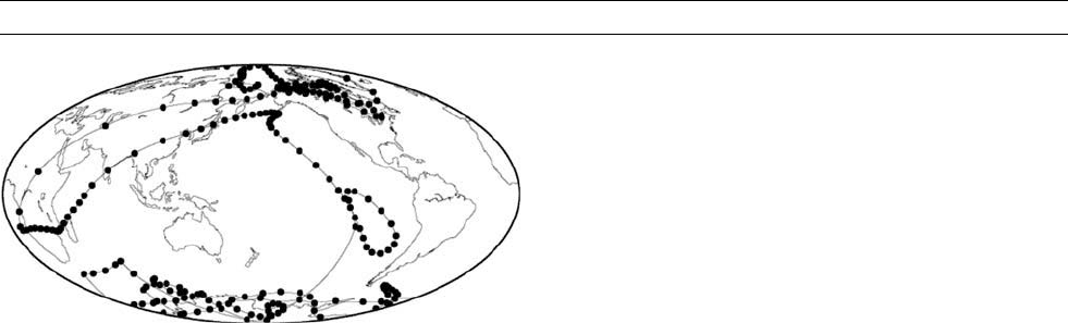
Figure G29 The Matuyama-Brunhes polarity transition obtained

from North Atlantic deep-sea sediments (Channell and Lehman,

1997) shown as the path the VGP positions track along as the

field gradually changes from reverse polarity (VGPs near the

south geographic pole) to normal polarity (VGPs near the north

geographic pole).

326 GEOMAGNETIC POLARITY REVERSALS, OBSERVATIONS

has been found for a remagnetization of intermediate directions in a

sediment record of an excursion (Coe and Liddicoat, 1994).

Yet another controversy regards how fast the magnetic field can

change during a reversal. The reversal recorded by lava flows at Steens

Mountain, Oregon provides evidence that the transitional field may

change as fast as degrees per day (Coe and Prevot, 1989; Coe et al.,

1995). This rate is extremely fast and in fact is thought to be too fast

(Figure G30). This is because the electrical conductivity of Earth’s

mantle filters field changes produced by the dynamo and should limit

just how fast the dynamo-produced field can change at Earth’s surface.

The evidence for the rapid changes comes from magnetizations

recorded within a single lava flow. The magnetizations differ with

position in the flow. Using cooling rate estimates for the flow, the rate

at which the field was changing can be estimated. Despite an intensive

effort, no evidence has been found to suggest that the different magne-

tizations result from differences in the magnetic minerals that record

the field.

These controversies will likely be resolved as additional polarity

transition records are obtained from a greater geographic distribution

and as records of older reversals are obtained. These records will help

solve the mystery of what happens during a polarity reversal, and that

knowledge will in turn help us understand what it is about Earth that

gives rise to this fascinating feature of our magnetic field.

Bradford M. Clement

Bibliography

Cande, S.C., and Kent, D.V., 1995. Revised calibration of the geomag-

netic polarity timescale for the Late Cretaceous and Cenozoic.

Journal of Geophysical Research, 100: 6093–6095.

Channell, J.E.T., and Lehman, B., 1997. The last two geomagnetic

polarity reversals recorded in high-deposition-rate sediment drifts.

Nature, 389: 712–715.

Clement, B.M., 1991. Geographical distribution of transitional

VGPs: evidence for non-zonal equatorial symmetry during the

Matuyama-Brunhes geomagnetic reversal. Earth and Planetary

Science Letters, 104:48–58.

Clement, B.M., 2004. Dependence of the duration of geomagnetic

polarity reversal on site latitude. Nature, 428(6983): 608–609.

Coe, R.S., and Liddicoat, J.C., 1994. Overprinting of natural magnetic

remanence in lake sediments by a subsequent high intensity field.

Nature, 367:57–59.

Coe, R.S., and Prevot, M., 1989. Evidence suggesting extremely rapid

field variation during a geomagnetic reversal. Earth and Planetary

Science Letters, 92: 292–298.

Coe, R.S., Prevot, M., and Camps, P., 1995. New evidence for extra-

ordinarily rapid change of the geomagnetic field during a reversal.

Nature, 374: 687–692.

Gee, J.S., Tauxe, L., Barge, E., Peirce, J.W., Weissel, J.K., Taylor, E.,

Dehn, J., Driscoll, N.W., Farrell, J.W., Fourtanier, E., Frey, F.A.,

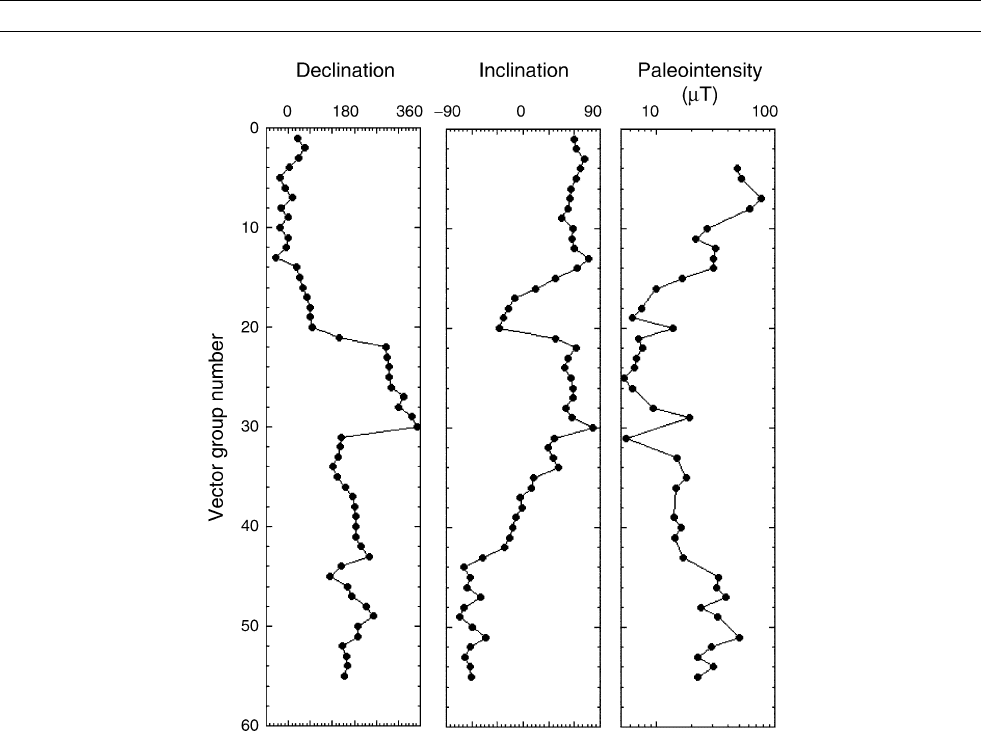
Figure G30 A record of a polarity reversal recorded in lava flows at Steens Mountain, Oregon (Mankinen et al., 1985; Prevot et al.,

1985). The changes in magnetization through the reversal are shown here plotted as declination, inclination, and paleointensity in

stratigraphic sequence of similar magnetization vectors. The data are plotted versus vector group number because it is assumed that

successive flows exhibiting the same magnetizations were extruded rapidly and represent multiple records of the same field and do not

necessarily represent times when the field was not changing.

GEOMAGNETIC POLARITY REVERSALS, OBSERVATIONS 327

Gamson, P.D., Gibson, I.L., Janecek, T.R., Klootwijk, C.T.,

Lawrence, J.R., Littke, R., Newman, J.S., Nomura, R., Owen,

R.M., Pospichal, J.J., Rea, D.K., Resiwati, P., Saunders, A.D., Smit,

J., Smith, G.M., Tamaki, K., Weis, D., and Wilkinson, C., 1991.

Lower Jaramillo polarity transition records from the equatorial

Atlantic and Indian oceans: Proceedings of the Ocean Drilling Pro-

gram, Scientific Results, 121:377–391.

Hillhouse, J.A., and Cox, A., 1976. Brunhes-Matuyama polarity tran-

sition. Earth and Planetary Science Letters, 29:51–64.

Hoffman, K.A., 1984. A method for the display and analysis of transi-

tional paleomagnetic data. Journal of Geophysical Research, 137:

6285–6292.

Hoffman, K.A., 1991. Long-lived transitional states of the geomag-

netic field and the two dynamo families. Nature, 354: 273–277.

Hoffman, K.A., 1992. Dipolar reversal states of the geomagnetic field

and core-mantle dynamics. Nature, 359: 789–794.

Laj, C., Mazaud, A., Weeks, R., Fuller, M., and Herrero-Bervera, E.,

1991. Geomagnetic reversal paths. Nature, 351: 447.

Love, J.J., and Mazaud, A., 1997. A database for the Matuyama-

Brunhes magnetic reversal. Physics of the Earth and Planetary

Interiors, 103: 207–245.

Mankinen, E.A., Prevot, M., Gromme, C.S., and Coe, R.S., 1985.

The Steens Mountain (Oregon) geomagnetic polarity transition.

I. Directional history, duration of episodes, and rock magnetism.

Journal of Geophysical Research, 90: 10393–10417.

Merrill, R.T., and McFadden, P.L., 1999. Geomagnetic polarity transi-

tions. Reviews of Geophysics, 37: 201–226.

Prevot, M., Mankinen, E.A., Coe, R.S., and Gromme, C.S., 1985. The

Steens Mountain (Oregon) geomagnetic polarity transition. 2. Field

intensity variations and discussion of reversal models. Journal of

Geophysical Research, 90: 10417–10448.

Singer, B.S., and Pringle, M.S., 1996. Age and duration of the

Matuyama-Brunhes geomagnetic polarity reversal for

Ar/

incremental heating analyses of lavas. Earth and Planetary Science

Letters, 139:47–61.

Tauxe, L., 1993. Sedimentary records of relative paleointensity of the

geomagnetic field: theory and practice. Reviews of Geophysics, 31:

319–354.

Cross-references

Core-Mantle Boundary Topography, Implications for Dynamics

Core-Mantle Boundary Topography, Seismology

Core-Mantle Boundary, Heat Flow Across Geodynamo

Geodynamo, Dimensional Analysis and Timescales

Geodynamo, Numerical Simulations

Magnetic Anomalies, Marine

Nondipole Field

Reversals, Theory

GEOMAGNETIC POLARITY TIMESCALES

Marine magnetic anomaly record

It is well established that Earth’s magnetic field has alternated fre-

quently but irregularly between two opposing polarity states for at

least most of the Phanerozoic. Older rocks of Proterozoic age that dis-

play both polarity states are also known, but whether they correspond

to reversals of a dipole field is less firmly established. The time inter-

val during which geomagnetic polarity remains constant is called a

polarity chron; long episodes of continuous reversal behavior are

called superchrons. The polarity equivalent to the present state is

referred to as “normal” and the opposite state as “reversed.”

The history of geomagnetic polarity is derived from two sources: the

interpretation of lineated marine magnetic anomalies, and magnetic

polarity stratigraphy in continuous sedimentary sequences and radio-

metrically dated igneous rocks. Since the Late Jurassic, when the cur-

rent phase of seafloor spreading began, these records support and

confirm each other. The geomagnetic polarity timescale (GPTS) is

most reliable for this time. It is divided into two sequences of alternat-

ing polarity, the younger covering the Late Cretaceous and Cenozoic,

and the older corresponding to Early Cretaceous and Late Jurassic

time. The reversal sequences are referred to as the C-sequence and

M-sequence, respectively. They are separated in the oceanic record

by the Cretaceous Quiet Zone in which lineated magnetic anomalies

are absent. It appears that Earth’s magnetic field did not reverse polar-

ity during this time interval, which is referred to as the Cretaceous nor-

mal polarity superchron (CNPS). Prior to the Late Jurassic only the

polarity record preserved in rocks is available. Knowledge of older

geomagnetic polarity history is patchy and, despite some excellent

magnetostratigraphic results, largely unconfirmed.

Construction and identification of a polarity

chron sequence

Although the pioneering studies of geomagnetic polarity were carried

out on radiometrically dated lavas, the marine magnetic anomaly

record provides the most extensive, detailed and continuous record

of reversal history and forms the basis of all GPTS covering the last

160 Ma of the Earth history. The appearance of lineated large ampli-

tude, long wavelength marine magnetic anomalies (Figure G31)

depends on the latitude and direction of the corresponding measure-

ment profile. The first step in constructing a GPTS thus consists of

interpreting the anomalies as a block model of alternating magnetiza-

tion of the oceanic crust responsible for the anomalies. The polarity

pattern is used to correlate coeval segments of different profiles and

to obtain an optimized model that minimizes local variations in spread-

ing rate on any given profile. The ensuing composite block model con-

stitutes a polarity sequence in which the distances between the block

boundaries are proportional to the relative lengths of the polarity

chrons. No consideration is usually given to the finite duration of a

polarity transition, which is thought to last about 4–6 ka (Clement

and Kent, 1984). This time is included in the lengths of polarity

chrons, which are measured between the midpoints of polarity transi-

tions. This simplification is generally acceptable but it may be proble-

matic for accurately describing short polarity chrons for which the

transitional time may be an appreciable fraction of the duration of

the chron.

The anomalies are identified by numbering them in increasing order

away from the spreading axis. In the C-sequence the positive magnetic

anomalies, corresponding to normal polarity, are numbered and pre-

ceded by the letter “C,” as anomalies C18, C29, etc. The M-sequence

oceanic crust in the North Pacific Ocean was magnetized south of the

equator but plate motion has brought it into the northern hemisphere.

The positive anomalies, identified by the letter “M” as anomalies

M0, M13, etc., correspond to reversely magnetized crust. To reconcile

the two numbering schemes, adjacent normally and reversely polarity

chrons are paired, so that the younger member has normal polarity.

Thus marine magnetic anomaly C15 is associated with polarity chrons

C15n and C15r.

To obtain an optimized global model of polarity, which then

becomes the polarity sequence for a GPTS, block models for different

spreading centers must be compared, stretched, and squeezed differen-

tially. The matching of block models may be visual or more sophisticated.

To form an optimized record of the C-sequence of polarity Cande and

Kent (1992a) used nine rotation poles to stack polarity records on contem-

poraneous profiles and determine relative widths of crustal blocks for the

modeled reversal sequence. Before a timescale can be generated, the opti-

mized polarity sequence must be dated. Biostratigraphic stage boundaries

or other dated levels are correlated by magnetostratigraphy to the polarity

328 GEOMAGNETIC POLARITY TIMESCALES

sequence. Intervening reversal boundaries between the calibration levels

are dated by linear interpolation and older boundaries by extrapolation.

The largest sources of error in this dating are the “absolute” ages asso-

ciated with the tie-levels. The relative lengths of the polarity chrons,

derived from a crustal block model that assumes constant spreading rate,

are known more accurately.

Cenozoic and Late Cretaceous GPTS

The pioneering efforts to determine a GPTS were carried out on mar-

ine magnetic anomalies at actively spreading oceanic ridge systems.

Heirtzler et al. (1968), hereafter referred to as HDHPL68, derived a

GPTS from the present time to the Late Cretaceous by matching pro-

files in different oceans to a reference profile in the South Atlantic,

which was judged to be the most likely to have a constant spreading

rate. The spreading rate at the South Atlantic Ridge was estimated

by correlating distances to young reversals with radiometrically dated

reversals from lava sequences. By assuming this spreading rate to be

constant, the distance of a polarity reversal from the ridge could be

converted to age. However, it was later found that the magnetic

anomalies composing anomaly C14 in HDHPL68 were not reproduci-

ble in other oceans and thus did not correspond to polarity intervals;

moreover, the HDHPL68 timescale did not cover the full range of

older anomalies following the Cretaceous Quiet Interval. Improved,

extended, and modified, the HDHPL68 timescale served as the basis

for several subsequent versions of the GPTS for this time interval (Fig-

ure G32). Magnetostratigraphic correlation of the Cretaceous–

Tertiary boundary to the upper part of chron C29r in a continental

exposure of marine limestones (Alvarez et al., 1977) provided a way

of associating age with the older end of the reversal sequence and

resulted in improved calibration of the C-sequence GPTS. The magne-

tostratigraphy also confirmed that the C-sequence began at C33r, as

termination of the CNPS. Together with more detailed analysis of

the oceanic record, this led to a more complete and accurate GPTS

(LaBrecque et al., 1977), hereafter LKC77.

The number of stage boundaries now tied to the polarity record led

Lowrie and Alvarez (1981) to propose a modification of the GPTS.

They assumed the polarity sequence in LKC77 and best estimates of

the “absolute” ages for 11 tie-levels that correlated the stratigraphic

and marine magnetic polarity records. Disregarding the effects on sea-

floor spreading rates they stretched and squeezed the polarity record

between the tie-points and obtained a new GPTS. The ensuing time-

scale resulted in a history of seafloor spreading characterized by sud-

den large changes in spreading rate. To avoid this, Harland et al.

(1982) modified the ages of tie-points and obtained a GPTS that gave

a smoother seafloor spreading record. One of the most important uses

of a GPTS is now recognized to be the ability to attach numeric ages

to faunal appearances and extinctions. Berggren et al. (1985) and

Harland et al. (1990) produced GPTS versions in which the biostrati-

graphy was well tied to the magnetic polarity record, which was

derived from that of LKC77.

Cande and Kent (1992a) carried out a detailed reevaluation of the

C-sequence marine magnetic anomalies and improved the definitions

of the corresponding oceanic block models, resulting in adjustments of

the relative lengths of polarity chrons. They associated ages with the

improved polarity sequence by fitting a cubic spline curve to nine dated

correlation points. In so doing they used a nonstandard age for the

Cretaceous-Tertiary boundary. An updated version of their timescale

(Cande and Kent, 1995), hereafter referred to as CK95, is the current

reference GPTS for the Late Cretaceous and Cenozoic. An archive

of Cenozoic-Late Cretaceous timescales has been assembled by Mead

(1996).

The Cretaceous normal polarity superchron

The C-sequence and M-sequence polarity chrons are separated by the

CNPS. Using the nomenclature for labeling chrons, this might be

called C34n or M0n, but it is customary to designate it separately from

the adjacent sequences. In the marine magnetic anomaly record the

CNPS corresponds to regions of oceanic crust referred to as the Cre-

taceous Quiet Zone, in which magnetic anomalies, although present,

are not lineated. It is believed to represent an interval of time, from

about 121 to 83 Ma ago, in which the geomagnetic field had a consis-

tent normal polarity. Despite magnetostratigraphic and deep-tow inves-

tigations to find polarity reversals within this 38 Ma interval, there is

no incontrovertible evidence of them. The absence of polarity changes

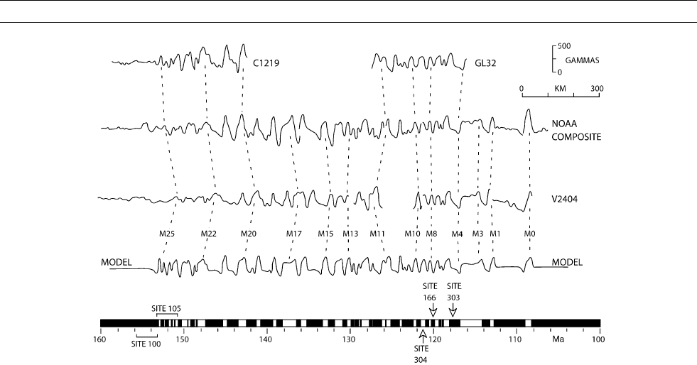
Figure G31 Marine magnetic profiles, correlation tie-lines, and block model of the polarity of oceanic crustal magnetization (black,

normal; white, reverse) for M-sequence anomalies in the North Pacific (after Larson and Hilde, 1975).

GEOMAGNETIC POLARITY TIMESCALES 329

in the CNPS may imply a special behavior of the geodynamo. A few

very long polarity chrons, lasting several million years each, are found

adjacent to the CNPS.

Early Cretaceous and Late Jurassic GPTS

The oldest regions of oceanic crust characterized by lineated magnetic

anomalies were formed during the Late Jurassic. The Phoenix, Japa-

nese, and Hawaiian lineations are found in the Western Pacific, and

the Keathley lineations in the western North Atlantic. Larson and

Pitman (1972) identified and correlated these sets of anomalies, num-

bering them from M1 to M22 in order of increasing age. They realized

that the three sets of Pacific lineations were inverted with respect to the

Keathley sequence. The North Pacific oceanic crust had been magne-

tized south of the magnetic equator, so that positive anomalies are

now found over reversely magnetized crust. Larson and Hilde (1975)

refined the reversal record for the Hawaiian lineations, resolving addi-

tional anomalies, adding a younger anomaly M0, and extending the

older anomaly record to M25 ( Figure G31). They dated their timescale

(LH75) by estimating the age of magnetic basement at drillholes of the

Deep Sea Drilling Project from the paleontological ages of the oldest

calcareous fossils found in the holes. The magnetic reversal block model

was derived for the Hawaiian lineations, but the ages were determined

for sites on other lineation sets and correlated by the magnetic polarity

pattern to the Hawaiian set.

The LH75 polarity sequence has formed the basis for subsequent mod-

ifications and improvementsto the M-sequence GPTS (FigureG33). Later

versions (Kent and Gradstein, 1985; Harland et al., 1990) are somewhat

better dated, but still rely on bottom ages in groups of drillholes near the

ends of the sequence. A new Hawaiian block model with an optimized

approximation to a constant spreading rate was derived by Channell

et al. (1995) after critical comparison of block models for the Hawaiian,

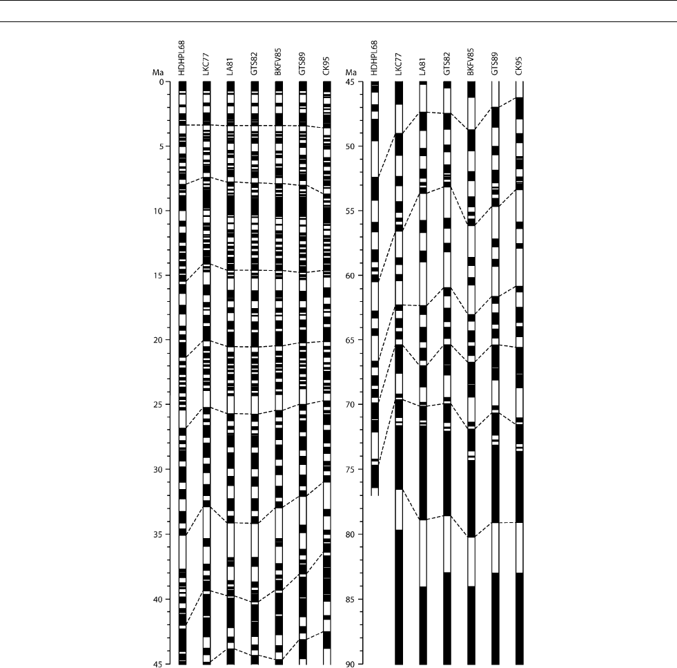
Figure G32 Evolution of the geomagnetic polarity timescale for the Cenozoic and Upper Cretaceous. The authors of individual

C-sequence models are as follows: HDHPL68, Heirtzler et al. (1968); LKC77, LaBreque et al . (1977); LA81, Lowrie and Alvarez (1981);

GTS82, Harland et al. (1982); BKFV85, Berggren et al. (1985); GTS89, Harland et al. (1990); CK95, Cande and Kent (1995).

330 GEOMAGNETIC POLARITY TIMESCALES

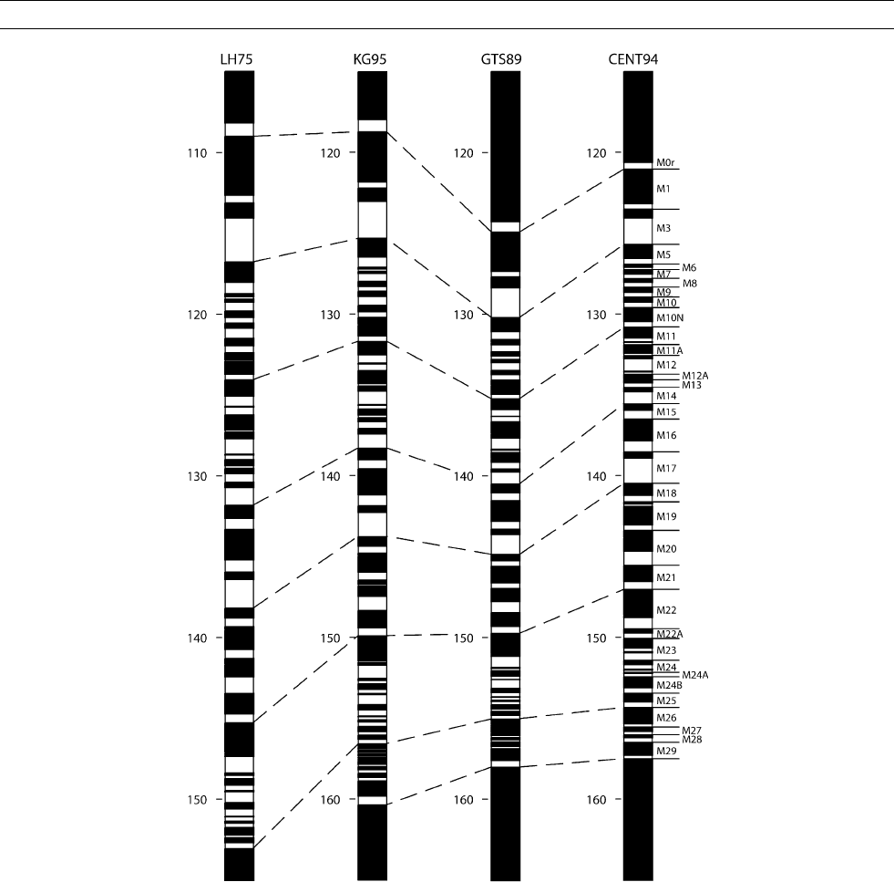
Japanese, Phoenix, and Keathley lineations. This model (CENT94), cov-

ering magnetic polarity chrons CM0r to CM29r, is probably the optimum

current GPTS for the M-sequence anomalies.

Oceanic crust older than chron CM25r was thought to be free of

lineated magnetic anomalies and was labeled the Jurassic Quiet Zone

by analogy to the Cretaceous equivalent. However, magnetic lineations

with low amplitude were subsequently identified in the youngest part

of this Quiet Zone, extending the polarity sequence to CM29r (Cande

et al., 1978). These weaker old anomalies are related to oceanic crust

whose magnetization decreases with increasing age. Even older

anomalies, with short wavelengths and low amplitudes, have been

detected within the Jurassic Quiet Zone, both from aeromagnetic pro-

files (Handschumacher et al., 1988) and from deep-towed magnet-

ometer surveys (Sager et al., 1998). Their origin is as yet uncertain.

They may have been formed during an episode of high reversal

frequency, in which case they would extend the M-sequence from

CM29r to CM41r. This would imply that the Jurassic Quiet Zone is

different in origin from the Cretaceous Quiet Zone, in which no rever-

sals are thought to have occurred. However, the polarity pattern corre-

sponding to these anomalies has not been established definitively and

the reversal sequence has not been confirmed independently by mag-

netostratigraphy. It is possible that the anomalies may be due to fluc-

tuations of paleomagnetic field intensity, as suggested to explain low

amplitude, short wavelength anomalies in the Cenozoic (Cande and

Kent, 1992b).

Early Juras sic and Triassic GPTS

The record of geomagnetic polarity prior to the onset of seafloor

spreading is much less well known. In the absence of a marine

Figure G33 Evolution of the geomagnetic polarity timescale for the Early Cretaceous and Late Jurassic. The authors of individual

M-sequence models are as follows: LH75, Larson and Hilde (1975); KG85, Kent and Gradstein (1985); GTS89, Harland et al. (1990);

CENT94, Channell et al. (1995).

GEOMAGNETIC POLARITY TIMESCALES 331

magnetic anomaly record, the GPTS must be pieced together from magne-

tostratigraphic results. This is a large undertaking. Changes of sedimenta-

tion rate within a given depositional basin or from one basin to another can

strongly modify the “fingerprint” pattern of reversals that is essential for

correlation. Investigations in marine limestones of Middle and Early

Jurassic age have identified magnetozones, but these have only rarely

been confirmed by other magnetostratigraphic results.

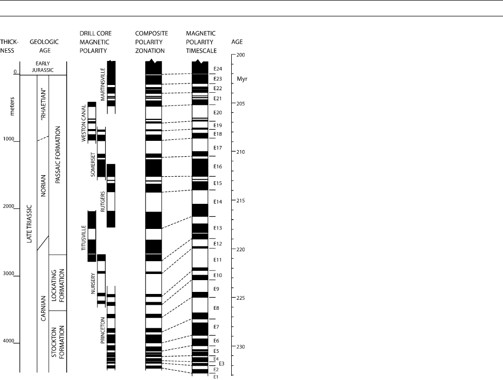
Kent et al. (1995) determined detailed magnetostratigraphies in

overlapping drillholes through continental redbeds of Late Triassic

age in the Newark basin. They matched the individual records strati-

graphically to produce a composite geomagnetic polarity record (Fig-

ure G34). The sediments displayed lithological variations related to

cyclical changes in Earth’s orbital parameters, of which the 400 ka

fluctuation of orbital eccentricity was prominent. Kent and Olsen

(1999) used this Milankovitch cycle to convert the polarity sequence

to a GPTS (Figure G34), assuming an “ absolute ” age of 202 Ma for

the Jurassic-Triassic boundary. The Newark section currently serves

as the standard of reference for the history of geomagnetic polarity

in the Late Triassic.

William Lowrie

Bibliography

Alvarez, W., Arthur, M.A., Fischer, A.G., Lowrie, W., Napoleone, G.,

Premoli Silva, I., and Roggenthen, W.M., 1977. Upper Cretaceous-

Paleocene magnetic stratigraphy at Gubbio, Italy. V. Type section

for the Late Cretaceous-Paleocene geomagnetic reversal time scale.

Geological Society of America Bulletin, 88:383–389.

Berggren, W.A., Kent, D.V., Flynn, J.J., and Van Couvering, J.A.,

1985. Cenozoic geochronology. Geological Society of America

Bulletin, 96: 1407–1418.

Cande, S.C., and Kent, D.V., 1992a. A new geomagnetic polarity time

scale for the Late Cretaceous and Cenozoic. Journal of Geophysi-

cal Research, 97: 13917–13951.

Cande, S.C., and Kent, D.V., 1992b. Ultra-high resolution marine

magnetic anomaly-profiles: a record of continuous paleointensity

variations? Journal of Geophysical Research, 97: 15075–15083.

Cande, S.C., and Kent, D.V., 1995. Revised calibration of the geomag-

netic polarity timescale for the Late Cretaceous and Cenozoic.

Journal of Geophysical Research, 100: 6093–6095.

Cande, S., Larson, R.L., and LaBrecque, J.L., 1978. Magnetic linea-

tions in the Pacific Jurassic quiet zone. Earth and Planetary

Science Letters, 41: 434–440.

Channell, J.E.T., Erba, E., Nakanishi, M., and Tamaki, K., 1995. Late

Jurassic-Early Cretaceous time scales and oceanic magnetic anom-

aly block models. In Berggren, W.A., Kent D.V., Aubry, M., and

Hardenbol, J. (eds.), Geochronology, Timescales, and Global Strati-

graphic Correlation. Tulsa, Oklahoma: SEPM Special Publication,

pp. 51–64.

Clement, B.M., and Kent, D.V., 1984. Latitudinal dependency of geo-

magnetic polarity transition durations. Nature, 310: 488–491.

Handschumacher, D.W., Sager, W.W., Hilde, T.W.C., and Bracey,

D.R., 1988. Pre-Cretaceous evolution of the Pacific plate and

extension of the geomagnetic polarity reversal time scale with

implications for the origin of the Jurassic “Quiet Zone”. Tectono-

physics, 155: 365–380.

Harland, W.B., Cox, A.V., Llewellyn, P.G., Pickton, C.A.G., Smith,

A.G., and Walters, R., 1982. A Geologic Time Scale. Cambridge:

Cambridge University Press, 131 pp.

Harland, W.B., Armstrong, R.L., Cox, A.V., Craig, L.E., Smith, A.G.,

and Smith, D.G., 1990. A Geologic Time Scale 1989. Cambridge:

Cambridge University Press, 263 pp.

Heirtzler, J.R., Dickson, G.O., Herron, E.M., Pitman, W.C. III, and

Le Pichon, X., 1968. Marine magnetic anomalies, geomagnetic

field reversals and motions of the ocean floor and continents.

Journal of Geophysical Research, 73:2119–2136.

Kent, D.V., and Gradstein, F.M., 1985. A Cretaceous and Jurassic geo-

chronology. Geological Society of America Bulletin, 96:1419–1427.

Kent, D.C., and Olsen, P.E., 1999. Astronomically tuned geomagnetic

polarity timescale for the Late Triassic. Journal of Geophysical

Research, 104: 12,831–12,841.

Kent, D.V., Olsen, P.E., and Witte, W.K., 1995. Late Triassic-Earliest

Jurassic geomagnetic polarity sequence and paleolatitudes from

drill cores in the Newark rift basin, eastern North America. Journal

of Geophysical Research, 100: 14965–14998.

LaBrecque, J.L., Kent, D.V., and Cande, S.C., 1977. Revised magnetic

polarity timescale for Late Cretaceous and Cenozoic time. Geology,

5:330–335.

Larson, R.L., and Hilde, T.W.C., 1975. A revised time scale of mag-

netic reversals for the Early Cretaceous and Late Jurassic. Journal

of Geophysical Research, 80: 2586–2594.

Larson, R.L., and Pitman, W.C. III, 1972. World-wide correlation of

Mesozoic magnetic anomalies, and its implications. Geological

Society of America Bulletin, 83: 3645–3662.

Lowrie, W., and Alvarez, W., 1981. One hundred million years of geo-

magnetic polarity history. Geology, 9: 392–397.

Figure G34 Construction of a GPTS for the Late Triassic based on

overlapping magnetostratigraphies from drillholes in the Newark

Basin, USA (after Kent et al., 1995). The GPTS is that of Kent and

Olsen (1999), calibrated by astrochronological dating of the

magnetozones.

332 GEOMAGNETIC POLARITY TIMESCALES

Mead, G.A., 1996. Correlation of Cenozoic-Late Cretaceous geomag-

netic polarity timescales: an Internet archive. Journal of Geophysi-

cal Research, 101: 8107–8109.

Sager, W.W., Weiss, C.J., Tivey, M.A., and Johnson, H.P., 1998.

Geomagnetic polarity reversal model of deep-tow profiles from

the Pacific Jurassic Quiet Zone. Journal of Geophysical Research,

103: 5269–5286.

Cross-references

Crustal Magnetic Field

Geomagnetic Polarity Reversals

Geomagnetic Polarity Timescales

Magnetic Anomalies, Marine

Magnetic Surveys, Marine

Magnetostratigraphy

Paleomagnetism

Reversals, Theory

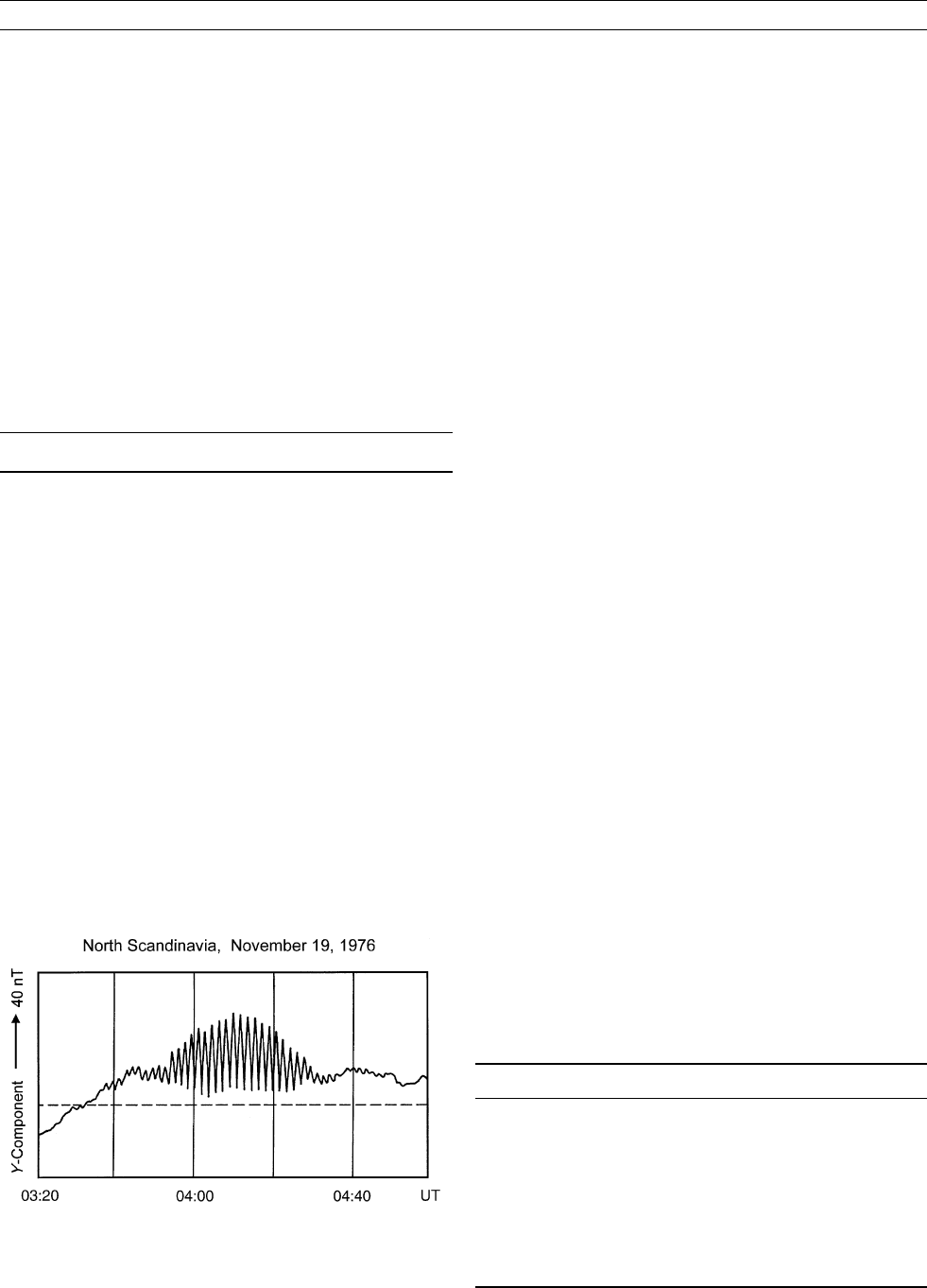
GEOMAGNETIC PULSATIONS

Geomagnetic pulsations or mircopulsations are ultralow frequency

(ULF) plasma waves in the Earth’s magnetosphere. These waves have

frequencies in the range 1 mHz to greater than 10 Hz and appear as

more or less regular oscillations in records of the geomagnetic field

(see Figure G35). Geomagnetic oscillations, or ULF pulsations as they

are also called, can also be identified in electric field measurements in

the ionosphere as well as observations of the electromagnetic field of

the magnetosphere as made onboard spacecraft.

The lower frequency pulsations have wavelengths comparable to

typical scale lengths of the entire magnetosphere. They may also be

interpreted as eigenoscillations of or standing waves in the magneto-

spheric systems. The higher frequency waves are usually identifiable

as proton ion-cyclotron waves in the magnetospheric plasma. The

amplitudes of the lower frequency pulsations can reach several tens

up to hundreds of nanotesla in the auroral zone region while the higher

frequency waves reach amplitudes of the order of a few nanotesla.

The first observation of a geomagnetic pulsation was published in

1861 by the Scottish scientist Balfour Stewart who identified quasisi-

nusoidal variations of the geomagnetic field in records of the Kew

observatory after the great magnetic storm that occurred in 1859.

The International Geophysical Year (1958–1959) with its large

number of coordinated geomagnetic field observations made available

a multitude of studies on ULF pulsations, stimulated the interest in this

type of geomagnetic field variation and created an active area of

research.

The classification scheme (Table G7) of the International Associa-

tion of Geomagnetism and Aeronomy (IAGA) distinguishes seven dif-

ferent types of geomagnetic pulsations based on their oscillation

period and appearance in magnetograms as almost continuous and

more irregular pulsations. The two classes, continuous pulsations

(Pc) and irregular pulsations (Pi), are usually divided into subclasses.

A more detailed overview of this morphological classification was

given by Jacobs (1970). Though this classification is still widely in

use it is somewhat outdated as the increased understanding of the phy-

sical nature and properties of geomagnetic pulsations allows a more in-

depth classification based on physical processes and generating

mechanisms. The long-period pulsations are at present interpreted as

magnetohydrodynamic waves while the short-period pulsations are

related to ion-cyclotron waves propagating in the magnetosphere. As

for many magnetospheric phenomena the solar wind provides the

energy for geomagnetic pulsations, partly directly, partly indirectly.

A direct energy source is plasma waves generated in the solar wind

and penetrating the magnetopause. A major source of these waves are

plasma instabilities in the upstream region of the near-Earth solar wind

where, for example, protons reflected at the magnetospheric bow

shock constitute an unstable particle distribution, generating a variety

of upstream waves. These waves are convected downstream toward

the magnetopause and couple through it into the magnetosphere.

Detailed investigations, however, indicate that the transmission of

hydromagnetic waves through the magnetopause is a rather inefficient

process. Only a small percentage of the energy of the upstream solar

wind waves couples to oscillations of the magnetosphere.

A more efficient, solar wind-driven process is the impulsive excita-

tion of plasma waves by sudden impulses from the solar wind. The

magnetosphere constitutes a kind of body capable of eigenoscillations.

It can be excited much like a bell. The British scientist Jim Dungey in

1954 was the first to analyze such eigenoscillations in more detail.

Assuming that the magnetospheric magnetic field is of dipole nature

only, he studied the magnetohydrodynamic equations of such a

dipole-magnetosphere filled with an ionized gas of spatially depending

mass density. The boundaries of this magnetosphere are the magneto-

pause and the ionosphere, where the geomagnetic field lines are

anchored much as strings of a violin are anchored between the pegs

and the tailpiece.

He derived the so-called Dungey equations, a set of partial differen-

tial equations describing the coupling between toroidal oscillations of

the fluid velocity field and the toroidal (poloidal) component of the

electric (magnetic) field oscillations in this dipole-magnetosphere. If

the excitation of the dipole-magnetosphere is axisymmetric, then the

toroidal components of these two fields are decoupled. This in turn

Figure G35 Geomagnetic pulsation of the Pc4 type, recorded at a

magnetic observatory in North Scandinavia. The y- or east-west

component of the geomagnetic field is displayed relative to a

quiet day record.

Table G7 The IAGA classification of geomagnetic pulsations

Name Period range (s)

Continuous

Pc1 0.2– 5

Pc2 5– 10

Pc3 10–45

Pc4 45–150

Pc5 150–600

Irregular

Pi1 1–40

Pi2 40–150

GEOMAGNETIC PULSATIONS 333

implies that individual field line shells are oscillating independent

from each other, much as different violin strings oscillate indepen-

dently. The oscillation period depends on Alfvén wave velocity along

the considered field line. Therefore geomagnetic pulsations can also be

used as a diagnostic tool for magnetospheric physics.

This is very much in accord with the observational finding that the

periods of geomagnetic pulsations in the Pc4–5 range decrease with

decreasing geomagnetic latitude. At lower latitudes the length of field

lines anchored between the northern and southern ionosphere is much

shorter than at higher latitudes, which causes a smaller oscillation per-

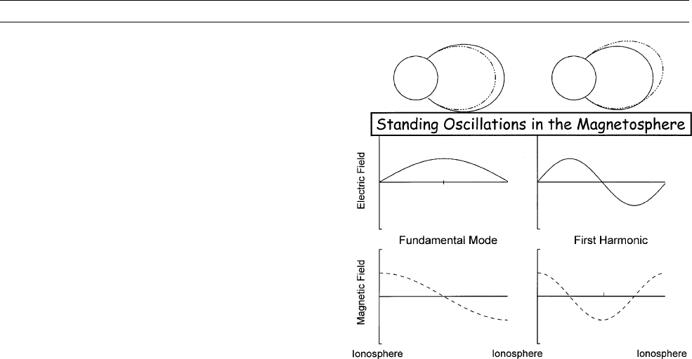
iod at low-latitudes. Geomagnetic oscillations can thus be viewed at as

standing field line oscillations with fundamental and higher harmonic

waves being generated (Figure G36).

Besides an impulsive excitation of geomagnetic pulsations the so-

called Kelvin-Helmholtz instability can drive magnetospheric magne-

tohydrodynamic waves. At the interface between the solar wind

plasma and the magnetosphere plasma, the so-called magnetopause,

strong shear flows exists. The solar wind plasma has to flow around

the magnetosphere along the magnetopause. Much as atmospheric

wind flow over a water surface can cause water waves the velocity

shear at the magnetopause destabilizes this boundary and causes sur-

face waves which are coupled into the magnetosphere. The energy

for these waves is drained out of the solar wind flow and maximum

instability of the magnetopause is expected at the flanks of the magne-

tosphere, which is in the dawn and dusk hours. Furthermore, the

unstable waves should propagate tailward that is they propagate east

at dusk and west at dawn. This is indeed observed in ground and satel-

lite observations of geomagnetic pulsations.

As the plasma density distribution is not uniform wave propagation

in the magnetosphere may lead to a very interesting physical effect,

field line resonance or resonant mode coupling. A Kelvin-Helmholtz

instability generated wave is a compressional magnetohydrodynamic

wave, which couples to a transverse oscillation, an Alfvén wave, at a

region in the magnetosphere where the surface wave’s period equals

the local eigenperiod of the toroidal field oscillation or Alfvén wave.

At this resonance point the oscillation magnitude maximizes and the

wave phase changes by 180



when crossing the resonant field line in

the radial direction. The physics of this resonant mode coupling

between a surface wave and a local eigenmodes is actually a tunneling

process (Southwood and Hughes, 1983).

Internal to the magnetosphere a variety of wave sources exist. Most

important is the ring current region with its energetic protons. Proton

distributions are usually nonthermal and tend to thermalize via interac-

tion with electromagnetic waves. These waves in turn can be generated

by plasma instabilities such as the so-called bounce-resonance or drift-

mirror instabilities (Samson, 1991; Walker, 2004).

The ring current region is also the source region of many of the Pc1-

Pc2 geomagnetic pulsations. During the expansive phase of magneto-

spheric substorms large numbers of energetic ions are injected from

the magnetotail into the inner magnetosphere where they drift west-

ward to create the substorm-enhanced ring current. These energetic

particle populations are highly unstable against the ion-cyclotron

instability and cause the generation of short-period geomagnetic pulsa-

tions (Kangas et al., 1998).

Once geomagnetic pulsations have been generated in the magne-

tosphere their energy must be dissipated somewhere. Most of this

dissipation occurs in the ionosphere where the pulsation-associated

electric fields cause current flow, which in turn leads to significant

Joule heating of the ionosphere. Local kinetic temperature increases

of several thousand Kelvin have been observed. Part of the wave

energy is also used to accelerate magnetospheric particles. Such

high-energy particles may subsequently hit the atmosphere where they

can cause aurora.

Much as the terrestrial magnetosphere also magnetospheres of other

planets, in particular those of Mercury, Jupiter, and Saturn exhibit

magnetic field oscillations comparable to geomagnetic pulsations

(Glassmeier et al., 1999). Magnetic pulsations of these magneto-

spheric systems have different properties than those at Earth due

to, for example, different spatial scales of the oscillating system.

Karl-Heinz Glaßmeier

Bibliography

Glassmeier, K.H., Othmer, C., Cramm, R., Stellmacher, M., and

Engebretson, M., 1999. Magnetospheric field line resonances: a

comparative planetology approach. Surveys in Geophysics, 20:

61–109.

Jacobs, J.A., 1970. Geomagnetic Micropulsations. Berlin: Springer-

Verlag.

Kangas, J., Guglielmi, A., and Pokhotelov, O., 1998. Morphology and

physics of short-period magnetic pulsations. Space Science

Reviews, 83: 435–512.

Samson, J.C., 1991. Geomagnetic pulsations and plasma waves in

the Earth’s magnetosphere. In Jacobs, J.A. (ed.), Geomagnetism,

Vol. 4. London: Academic Press, pp. 481– 592.

Southwood, D.J., and Hughes, W.J., 1983. Theory of hydromagnetic

waves in the magnetosphere. Space Science Reviews, 35: 301–366.

Walker, A.D.M. (ed.), 2004. Magnetohydrodynamic Waves in Geospace:

The Theory of ULF Waves and Their Interaction with Energetic Parti-

cles in the Solar-Terrestrial Environment. Philadelphia: Institute of

Physics Publishing.

Cross-references

Alfvén Waves

Ionosphere

Magnetohydrodynamic Waves

Magnetosphere of the Earth

Ring Current

Figure G36 Schematic representation of standing geomagnetic

field line oscillations. The perturbed field line is the dashed-dotted

line. The electric field always has a node in the ionosphere as

large electrical conductivity there shortcuts all electric potential

differences.

334 GEOMAGNETIC PULSATIONS

GEOMAGNETIC REVERSAL SEQUENCE,

STATISTICAL STRUCTURE

Introduction

It is now well recognized that the geomagnetic field is produced by

dynamo action within the molten iron in the outer core. This is a

dynamic process intimately linked to cooling of the core and the rapid

spin of the Earth. The equations governing the geodynamo, which

have to be solved jointly to obtain a full model of the process, are

Maxwell’s equations, Ohm’s law, the Navier-Stokes’ equation, the

continuity equation, Poisson’s equation, the generalized heat equation,

and the equation of state for the material in the outer core. This is a

complex, nonlinear set of equations, making it extraordinarily difficult

to obtain a full solution. However, the equations are even in H, the

magnetic field. That is, the equations are insensitive to the sign of

H, and so if H is a solution then so also is – H. We know from pre-

sent-day observations that the geomagnetic field can exist in a rela-

tively stable state in which the field at the Earth’s surface is

approximately that of a dipole with its axis almost parallel to the

Earth’s spin axis. Consequently we should expect that there is a similar

relatively stable solution, with the same statistical properties as the

field we observe today, that simply has the opposite polarity, that is,

the north and south poles are swapped. Hence, if there is a mechan-

ism for the field to move from one solution to the other, we should

expect to see reversals of the geomagnetic field. The solar magnetic

dynamo reverses regularly with a full period of about 22 years (see

Magnetic field of Sun), so we know that reversal is possible in other

self-sustaining dynamos. This then leaves open the question of how

we can tell whether the field has reversed polarity in geological time,

well before humans started to observe the field and its behavior.

By at least the late 18th century it was recognized that deviation of

magnetic compasses could occur because of nearby strongly magne-

tized rocks. The first observations that the magnetization in certain

rocks was actually parallel to the Earth’s magnetic field were made

independently by Delesse and Melloni. Folgerhaiter extended their

work but also studied the magnetization of bricks and pottery. He

argued that when a brick or pot was fired in the kiln then the remanent

magnetization it acquired on cooling provided a record of the direction

of the Earth’s magnetic field. With the wisdom of hindsight it is fairly

obvious that this would be the case. Volcanic rocks are heated well

above the Curie point so the magnetization is free to align with the

external magnetic field and becomes locked in as the rock cools. This

is known as a thermoremanent magnetization (TRM) (q.v.) and, in

extrusive volcanics, provides a record of the direction of the magnetic

field at that locality at a specific point in time.

There are several processes by which a rock will lock in a fossil record

of the ancient (or paleo) magnetic field. The fossil magnetism naturally

present is termed the natural remanent magnetization (NRM) (q.v.)and

its existence provides us with an opportunity to discover the direction of

the geomagnetic field over geological time. David in 1904 and Brunhes

in 1906 reported the first discovery of NRM that was roughly opposite

in direction to that of the present field and this led to the speculation that

the Earth’s magnetic field had reversed its polarity in the past. At that time

it was not recognized that the field was generated by a self-sustaining

dynamo in the outer core, so the possibility of reversal was more exciting

than it may seem from our perspective today. In 1926, Mercanton pointed

out that if the Earth’s field had in fact reversed itself in the past then

reversely magnetized rocks should be found in all parts of the world.

He demonstrated that this was indeed the case for Quaternary-aged rocks

around the world. The speculation gained further support when

Matuyama in 1929 observed reversely magnetized lava flows from the

past 1 or 2 Ma in Japan and Manchuria. However, doubts about the

validity of the field reversal hypothesis surfaced during the 1950s after

Néel presented theory that showed it was possible for samples to acquire

a magnetization antiparallel to the external field during cooling, a

process referred to as self-reversal. Shortly thereafter Nagata and Uyeda

found the first laboratory-reproducible self-reversing rock, the Haruna

dacite. Subsequently, it was recognized that self-reversal is relatively

rare and by the early 1960s it was accepted that the Earth’s magnetic field

has indeed reversed and that the phenomenon of field reversal has

occurred many times. An excellent history of this subject was given by

Glen (1982).

A critical component in our understanding of reversals was develop-

ment in the early 1960s of the K-Ar dating method, which made it pos-

sible to date young volcanic rocks with reasonable precision.

Consequently, it was possible to undertake systematic studies attempt-

ing to define the geomagnetic polarity timescale (GPTS) using joint

magnetic polarity and K-Ar age determinations on young lavas. As

data rapidly became available, it was established that rocks of the same

age had the same polarity of magnetization, helping to confirm that the

observed reversals of magnetization were indeed due to reversals of

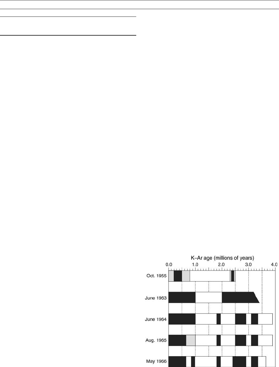
the geomagnetic field itself. A few of the earliest compilations, cover-

ing the years 1959–1966, of the GPTS for the past 4 Ma are shown in

Figure G37. Not surprisingly, when the field has the polarity that we

observe today, it is referred to as normal polarity, and the opposite

polarity is referred to as reverse polarity.

As already noted, the solar magnetic field has a periodic reversal,

and the first timescale put forward by Cox et al. (1963) appeared to

be consistent with geomagnetic reversals having a periodicity of about

1 Ma intervals. However, as new data appeared it rapidly became

apparent that there was no simple periodicity; some of the observed

polarity intervals were nearly a million years in length and some were

as short as 0.1 Ma. Furthermore, there did not appear to be any regular

pattern to these different lengths. This led to the suggestion that there

is a random component to the reversal process and, therefore, to inter-

est in the statistical structure of the geomagnetic reversal sequence.

It is extremely difficult to solve the geodynamo problem, that is, to

determine just how the geodynamo operates. Determination and under-

standing of the statistical structure of the geomagnetic reversal

sequence provides insight into the long-term dynamic process and in

so doing can provide powerful constraints on geodynamo models.

For example, the observation that the solar dynamo reverses with a

clear periodicity but the geodynamo reversal process appears random,

is probably a reflection of the different boundary conditions on the two

dynamos.

Figure G37 Early compilations of the GPTS. Black represents

normal polarity, white represents reversed polarity, and grey

indicates uncertain polarity. Abstracted with permission from Cox

(1969). ã American Association for the Advancement of Science.

GEOMAGNETIC REVERSAL SEQUENCE, STATISTICAL STRUCTURE 335