Gubbins D., Herrero-Bervera E. Encyclopedia of Geomagnetism and Paleomagnetism

Подождите немного. Документ загружается.

Cross-references

Core Convection

Core Turbulence

Core Viscosity

Core-Mantle Boundary Topography, Implications for Dynamics

Core-Mantle Coupling, Electromagnetic

Core-Mantle Coupling, Thermal

Core-Mantle Coupling, Topographic

Dynamo, Solar

Geodynamo

Geomagnetic Dipole Field

Harmonics, Spherical

Inner Core Rotation

Inner Core Seismic Velocities

Inner Core Tangent Cylinder

Magnetohydrodynamics

Reversals, Theory

Thermal Wind

Westward Drift

GEODYNAMO, SYMMETRY PROPERTIES

The behavior of any physical system is determined in part by its

symmetry properties. For the geodynamo this means the geometry of

a spinning sphere and the symmetry properties of the equations of

magnetohydrodynamics. Solutions have symmetry that is the same as,

or lower than, the symmetry of the governing equations and boundary

conditions. By “symmetry” here we mean a transformation T that takes

the system into itself. Given one solution with lower symmetry, we can

construct a second solution by applying the transformation T to it. Solu-

tions with different symmetry can evolve independently and are said to

be separable. If the governing equations are linear separable solutions

are also linearly independent: they may be combined to form a more gen-

eral solution. If the governing equations are nonlinear they may not be

combined or coexist but they remain separable. The full geodynamo

(q.v.) problem is nonlinear and separable solutions exist; fluid velocities

and magnetic fields with the same symmetry are linearly independent

solutions of the linear kinematic dynamo (q.v.) problem.

Symmetry considerations are important for both theory and observa-

tion. For example, solutions with high symmetry are easier to compute

than those with lower symmetry and are often chosen for that reason.

Time-dependent behavior of nonlinear systems (geomagnetic reversals

for example) may be analyzed in terms of one separable solution

becoming unstable to one with different symmetry (“symmetry break-

ing”). Observational applications include detection of symmetries in

the geomagnetic field. The axial dipole field has very high symmetry

but is not a separable solution of the geodynamo; it does, however,

belong to a separable solution with a particular symmetry about the

equator. Paleomagnetic data rarely have sufficient global coverage to

allow a proper assessment of the spatial pattern of the geomagnetic

field, but they can sometimes be used to discriminate between separ-

able solutions with different symmetries.

The sphere is symmetric under any rotation about its centre while

rotation is symmetric under any rotation about the spin axis. The sym-

metries of the spinning sphere are therefore any rotation about the spin

axis and reflection in the equatorial plane (Figure G15). This conflict

of spherical and cylindrical geometry lies at the heart of many of the

properties of rotating convection and the geodynamo. The equations

of magnetohydrodynamics (q.v.) are also invariant under rotation. They

are invariant under change of sign of magnetic field B (but not other

dependent variables) because the induction equation is linear in B

and the magnetic force and ohmic heating are quadratic in B. They

are also invariant under time translation.

The group of symmetry operations is Abelian because of the infinite

number of allowed rotations about the spin axis and time translations.

The full set of symmetry operations is found by constructing the group

table and using the closure property. The group table, including rotation

of p about the spin axis but no higher rotations, is shown in Table G6.

Note the additional symmetry operations O; these are combinations of

reflection in the equatorial plane and rotation about the spin axis; they

amount to reflection through the origin. Note also the subgroups formed

by (I,i)and(I,i,E

). These are fundamental to some analyses of

paleomagnetic data. Arbitrary time translation can be applied to any

symmetry to produce steady solutions that are invariant under transla-

tion, drifting solutions that are steady in a corotating frame, more com-

plicated time-periodic solutions that may vascillate or have reversing

magnetic fields, and solutions that change continually and are some-

times loosely called “chaotic.”

A word is needed about the behavior of vectors under reflection. A

vector is usually defined by its transformation law under rotation. An

axial or pseudovector (or tensor) changes sign on reflection whereas

a polar or true vector (or tensor) does not. A true scalar is invariant

under reflection, a pseudoscalar changes sign. Examples of true vec-

tors are fluid velocity and electric current. Examples of axial vectors

are angular velocity and magnetic field. The cross product changes

sign under reflection (to see this consider the simple case of the cross

product of two polar vectors); the curl also changes sign under reflec-

tion. Vectors v satisfying rv ¼ 0 are often represented in terms of

their toroidal and poloidal parts:

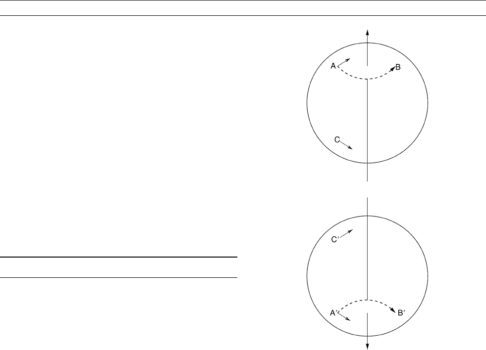
Figure G15 Reflection of a rotating sphere in a plane parallel to

the equator. A

are the reflections of the points A, B. The

reflected sphere turns in the same direction as the original sphere.

A vector is equatorial-symmetric (E

) if its value at C

appears as a

reflection as shown: it is E

if it appears with a change of sign.

306 GEODYNAMO, SYMMETRY PROPERTIES

v ¼rTr þrrPr;

if the toroidal part is a true vector the poloidal part will be a pseudo-

vector and vice versa because of the extra curl involved. Helicity,

v rv, is a pseudoscalar because vorticity changes sign under

reflection but velocity does not. Properties of true and pseudovectors

are used to determine the symmetry of individual terms in the govern-

ing equations and to find separable solutions.

The symmetry of solutions is reflected in their spherical harmonic

expansions. Potential fields with E

symmetry involve only harmonics

with l  m odd; E

fields have l  m even. The symmetries are

usually referred to as “dipole” and “quadrupole” families because of their

leading terms Y

(dipole) and Y

(quadrupole). The terminology is

somewhat unsatisfactory for two reasons: first, the equatorial dipole

is a member of the quadrupole family, and second the internal,

toroidal, field of each family has the opposite series to that of the

external, poloidal, field. Fields with P

symmetry have spherical

harmonic series with m even, P

have m odd. Solutions with

higher symmetry have series containing m differing by larger inte-

gers, for example P

has m multiples of 4.

The main use of symmetry properties in theoretical studies has so

far been restricted to reducing the complexity of the solution in order

to effect numerical solutions. For example, allowing only a “dipole

family,” or E

, solution halves the number of spherical harmonics

required to represent the solution (or, equivalently, the solution only

need be found in one hemisphere); P

halves it again. In practice solu-

tions with high symmetry may be poor dynamos and be more difficult

to compute, despite their apparent lack of spatial complexity, because

they require strong driving and involve small-scale magnetic fields.

The existence of a separable solution is no guarantee of maintaining

a magnetic field: B may still decay to zero. Thus axial symmetry is

an allowed symmetry but Cowling’s theorem (q.v.) shows that no

axisymmetric magnetic field can be sustained by dynamo action.

Kinematic dynamos ( q.v.) with axisymmetric fluid velocities have axi-

symmetric solutions that decay by Cowling’s theorem, but solutions

with lower symmetry, each proportional to expimf, can grow with

time. They do not form separable solutions of the full, dynamical,

dynamo problem because nonlinear terms in the equations couple the

modes to include many values of m. Bullard and Gellman (1954)

investigated an E

flow that also possessed a meridional plane of

symmetry, again to reduce the computational effort required for the

very small, early computer at their disposal. This last symmetry is

not an allowed separable solution of the full dynamo problem. The

lack of helicity imposed by this symmetry was later found to be the

reason for the failure of the Bullard-Gellman dynamo (q.v.).

The future may see further studies of dynamo behavior making

more use of symmetries. For example, reversals may be understood

in terms of the “dipole” E

solution becoming unstable to a “quadru-

pole” E

or an oscillatory solution. It was once suggested that reversals

may involve only the observed poloidal field, the larger internal toroi-

dal field retaining the same polarity, but this is unlikely because it vio-

lates the symmetry properties of the solution.

Symmetry properties have received more attention in observational

studies, particularly with paleomagnetic data (see Geomagnetic field,

asymmetries). The basic observation is that of an E

field, the dipole,

but equatorial symmetry appears to go beyond that of the dipole: the

main concentrations of magnetic field on the core-mantle boundary

form four lobes, two in the northern hemisphere and two in the south-

ern hemisphere, on closely similar longitudes (see Plate 10c). This basic

pattern is close to P

symmetry, but a nonaxisymmetric pattern would

only be of interest if it were long term. With homogeneous boundary con-

ditions we would expect the solution to drift without reference to any long-

itude, averaging to axial symmetry. This has been assumed in many

studies in the past; departures from axial symmetry would imply an effect

of inhomogeneity on the boundary, such as variable heat flux from the

core (see Core-mantle coupling, thermal). The lower mantle seismic

velocities suggest a P

pattern associated with subduction around the

Pacific rim, which could favor P

magnetic fields.

Further discussion of the theory is in Gubbins and Zhang (1993) and

of the data analysis in Merrill et al . (1996).

David Gubbins

Bibliography

Bullard, E.C., and Gellman, H., 1954. Homogeneous dynamos and

terrestrial magnetism. Philosophical Transactions of the Royal

Society of London, Series A, 247: 213–278.

Gubbins, D., and Zhang, K., 1993. Symmetry properties of the

dynamo equations for paleomagnetism and geomagnetism. Physics

of the Earth and Planetary Interiors, 75: 225–241.

Merrill, R.T., McElhinny, M.W., and McFadden, P.L., 1996. The Mag-

netic Field of the Earth. San Diego, CA: Academic Press.

Cross-references

Cowling’s Theorem

Core-Mantle Boundary Topography, Implications for Dynamics

Core-Mantle Coupling, Thermal

Dynamo, Bullard-Gellman

Dynamos, Kinematic

Geomagnetic Field, Asymmetries

Magnetohydrodynamics

Paleomagnetic Secular Variation

GEOMAGNETIC DEEP SOUNDING

Geomagnetic deep sounding (GDS) is the use of electromagnetic

induction methods to determine the electrical conductivity within the

Earth, working from observations of natural geomagnetic variations. It

is differentiated from the magnetotelluric method (q.v.) in employing only

the magnetic, and not the electric field. The term GDS is applied both to

global and to regional studies. The aim of global investigations is to deter-

mine the variation of electrical conductivity with depth. That of regional

studies is to map lateral differences in the conductivity of the crust and

upper mantle. The book by Rokityansky (1982) covers all aspects of

the subject. Weaver (1994) gives a detailed account of the theory.

Sounding the earth using natural geomagnetic

variations

A slowly varying magnetic field inside a uniform conductor (conduc-

tivity s and relative magnetic permeability m) satisfies the induction

equation:

Table G6 Multiplication table for a finite subgroup of spatial

symmetry operations for a buoyancy-driven dynamo in a rotating

sphere

IiE

iIE

IiO

iIO

IiE

iIE

Note: I, identity; i, field reversal; E

, reflection in equatorial plane; E

, reflection in

equatorial plane with change of sign of magnetic field; P

, rotation by p about spin

axis; and O , reflection in origin.

GEOMAGNETIC DEEP SOUNDING 307

B ¼ mm

The time-varying field induces eddy currents in the conductor which

flow so as to exclude the field from the deeper parts. The amplitude

of a spatially uniform field of frequency o falls to 1/e of its surface

value at the “skin-depth”:

2=omm

This expression provides a rough guide to the “sounding depth” which

might be expected of a particular frequency. However, the geometry of

the external source also restricts the depth or volume sampled by the

field. When induction effects are negligible, a field with spatial wave-

length l falls to 1/e of its surface value at depth l/2p. The basis of the

sounding method is to measure the Earth response at a range of fre-

quencies and/or source wavelengths. If the response of a one-dimen-

sional earth is known precisely either at all frequencies or all spatial

scales, the radial variation of conductivity is uniquely defined.

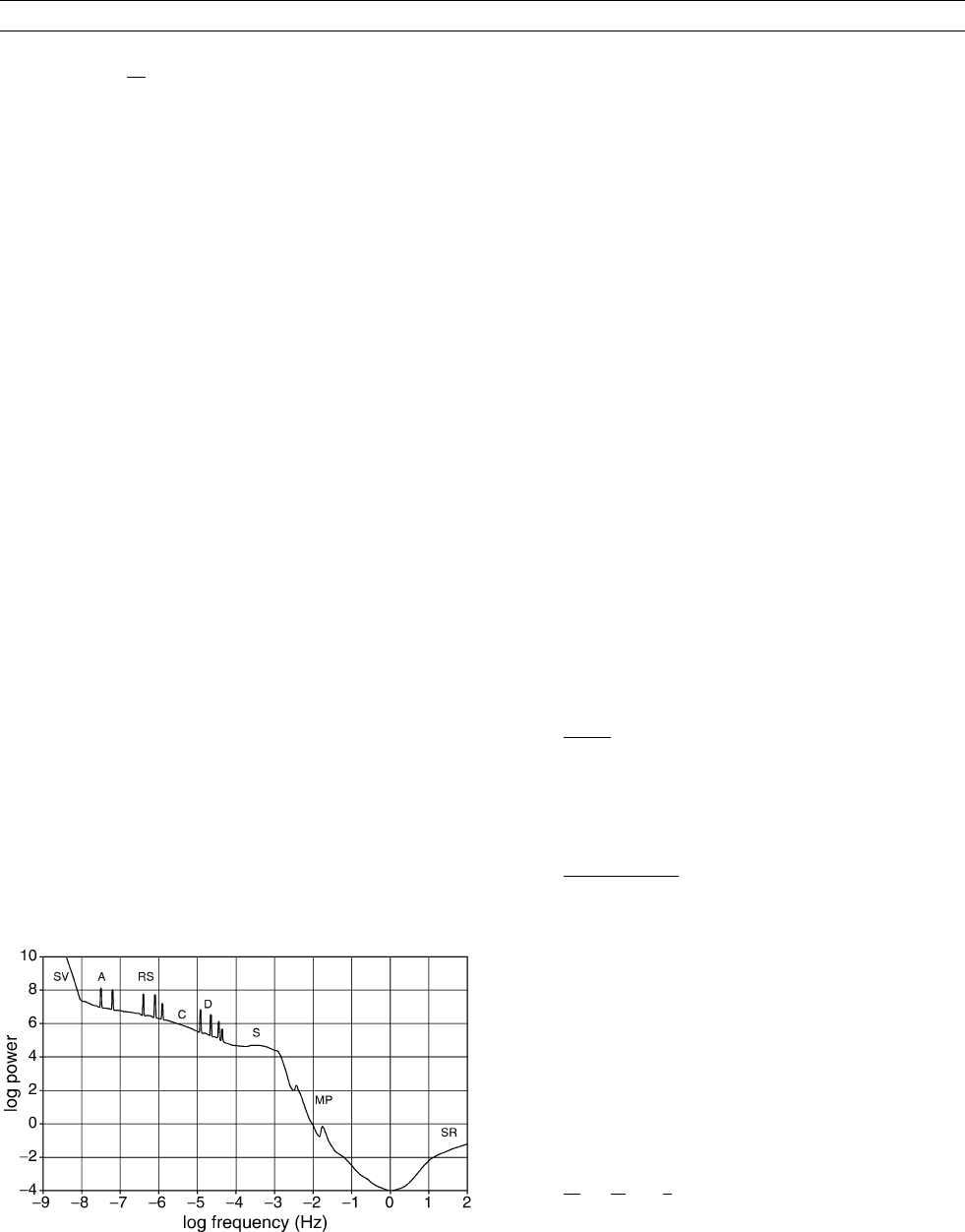
The geomagnetic variation spectrum

The frequency range of the externally generated electromagnetic spec-

trum (Figure G16) is extremely wide. The longest periods available

are associated with the solar cycle (11 or 22 years), and penetrate into

the lower mantle. Unfortunately, they are difficult to separate from the

purely internal variations with periods longer than 3 years generated

by the secular behavior of the dynamo. Much of the spectrum between

2 years and 2 days period comes from fluctuations in the total energy

of particles in the radiation belts, which drift in the geomagnetic field,

creating the ring current (q.v.). Because the current is located between

3 and 5 Earth radii, the field it creates at the Earth is relatively uni-

form, and its spatial structure can be represented by a small number

of zonal spherical harmonics (q.v.), of which the first (n ¼ 1) is much

the most important. Variations with this structure include the semiann-

ual line, the quasiperiodic harmonics at 27, 13.5, 9 days, etc., driven

by the Sun’s rotation and the persistence both of solar sources and sec-

tor structure in the solar wind, and the continuum. The annual varia-

tion, however, has a distinct spatial structure that is antisymmetric

about the equator, suggesting a seasonal driving force.

The daily variation and its harmonics are created by dynamo action

in the ionosphere, where thermal and gravitational tides move plasma

through the magnetic field. Their spatial structure can be adequately

represented by spherical harmonics up to degree n ¼ 4. The continuum

from a few days to a few minutes period originates in the current sys-

tems produced by geomagnetic storms. Their spatial structure is

complex, and in the auroral regions is localized as electrojets in the

ionosphere, and field-aligned currents connecting with the outer mag-

netosphere. Micropulsations are vibrations of geomagnetic field lines,

while Schumann resonances are oscillations of the Earth-ionosphere

waveguide excited by large-scale thunderstorm activity.

GDS—the global problem

Only magnetic observatories provide the record lengths required for

global sounding to depths of hundreds of kilometers. Because of

their poor distribution and insufficient numbers, only the smoother

fields are defined adequately. Temporary arrays of magnetometers

are deployed to map the more complex fields, and, in the absence of

conductivity anomalies, the field gradients can be used for local

soundings.

The determination of the vertical variation of conductivity is conve-

niently divided into two steps. The first is the measurement of the

response or transfer function (q.v.) which links the input—the external

part of the magnetic field—to the output—the internal part created

by the induced currents. The second is the inversion of the response

for the conductivity—discovering what can be inferred about s(r)

from the response and its associated errors.

Definition and determination of the response function

In global GDS, spherical harmonic functions (q.v.) are commonly used

to define the spatial structure of the field. The response Q

ðoÞ is the

ratio of the internal and external parts of the field at frequency o for a

spherical harmonic component of degree n and order m. An alternative

is the C response:

C ¼

=]r

The radial gradient of the vertical field is replaced by the horizontal

gradients of the horizontal components using the condition div

B ¼ 0. For plane earth geometry, and a smooth external field,

C ¼

=]x þ ]B

=]y

The C response has been favored in recent investigations because of its

intercomparability between global and local studies, and physical sig-

nificance as a penetration scale (its dimension is length).

The magnetic observatory network is inadequate for determining all

but the largest scale spatial structures. Instead of a full spherical har-

monic analysis, a simple spherical harmonic model is usually adopted,

based on what is known of the source. For periods between 2 years

and 2 days, a single zonal harmonic has been used, with the advantage

that the response can be computed from vertical (Z) and horizontal

(H) component records at a single observatory. The total potential of

internal (g

) and external (g

) sources for a spherical harmonic degree

n ¼ 1 and order m ¼ 0, is

O ¼

þ g



cos y

The corresponding components of the magnetic induction are

Z ¼B

ðr ¼ aÞ¼ 2g

þ g

cos y

H ¼B

ðr ¼ aÞ¼ g

þ g

sin y

Figure G16 Schematic representation of the natural geomagnetic

spectrum. SV, secular variation of the geodynamo; AV, annual

variation; RS, recurrent storms; C, continuum; D, daily variation;

S, storms and substorms; MP, micropulsations; SR, Schumann

resonance.

308 GEOMAGNETIC DEEP SOUNDING

The ratio of the vertical and horizontal components of the field, multi-

plied by tany, is itself a response (W

), which can be computed from

the component records by standard response estimation techniques:

tan y ¼

1  2Q



 1 þ Q



The major factors limiting the precision of response estimates are the

inadequacy of the source model and the influence of lateral variations

in conductivity. Attempts to incorporate these effects into response

determination and modeling are hampered by the limitations of the

observatory network.

Determination of the conductivity

The second step is the transformation of the electromagnetic response

data into a conductivity model. In the forward modeling approach

(q.v.), a conductivity distribution is selected either on the basis of inde-

pendent geophysical constraints, or for mathematical convenience. Its

response is computed and compared with the observations, and the

model parameters adjusted until a satisfactory fit is achieved. In the

inverse modeling method (q.v.), parameters which define the structure

are determined directly from the data. In practice, the two approaches

are more alike than at first appears. The class of structure, which is to

be the target of an inversion must be selected, and preferences about

the smoothness of models incorporated. A preliminary exploration of

simple models, for which the relationship between data and structure

is well understood, is always worthwhile.

Consider a model in which a perfectly conducting “core,” radius

r ¼ Ra, is surrounded by an insulating shell. The Q

response (to exci-

tation by ring current-generated fields) can be interpreted using the

spherical harmonic model to downward continue the field. The radial

component of the field in any source-free region is:

¼ g

2a

þ g



cos y;

and it must be zero at the surface of the perfect conductor. If B

¼ 0at

r ¼ Ra,

¼ g

¼ R

At 27 days period, the value of Q

is 0.3, which implies R ¼ 0.84, cor-

responding to a depth of 1000 km. This is a strong indication that the

conductivity rises steeply in the upper mantle.

The global electromagnetic response and global

conductivity distribution

The earliest determinations of the global response are summarized by

Chapman and Bartels (1940). Schuster, Chapman, Price, and Lahiri

used the daily variation and time-domain analyses of magnetic storms.

Conductivity models were restricted to those with analytical solu-

tions—a uniform core surrounded by a uniform insulator, and a power

law increase. With the arrival of the digital computer, Fourier trans-

form-based spectral analysis methods were introduced (Currie,

1966). The response could be determined at a continuous range of fre-

quencies, and it was possible to calculate the theoretical response of

arbitrary models (Banks, 1969). Recognition of the problems posed

by source complexity and lateral variations in conductivity led to more

robust response estimation and regionalization of the models (see

Constable, 1993). Weidelt and Parker (see Parker, 1983) clarified

the inverse problem and demonstrated that the best-fitting model for

any set of data was a set of thin conducting sheets. They also showed

how to construct more realistic models, which would, however, fit the

data less well. Constable applied their techniques to collated response

data. Olsen (1998, 1999) further refined both the response and models

for the European area.

There was early recognition of a steep rise in conductivity in the

400–800 km depth range to a value of 2 Sm

–1

(Figure G17). Later

work has made only minor differences. The major factors inhibiting

improvement are the inadequacy of the source model and the influence

of lateral variations in conductivity. Attempts to incorporate these

effects into response determination and modeling (Schultz and Zhang,

1994) are hampered by the nature of the observatory network. Satellite

observations may be one route to future progress.

GDS—mapping lateral variations in conductivity

Conductivity anomalies and their response

Outside the auroral zones, the externally generated part of the time-

varying magnetic field is uniform over hundreds of kilometers. If the

electrical conductivity were similarly uniform, the induced currents

would double the horizontal component of the external magnetic field

but cancel the vertical component. Such a conductivity structure, and

the fields associated with it, are referred to as “normal.” What addi-

tional “anomalous” fields are created when a region of different

conductivity—a conductivity “anomaly”—is embedded within the

normal structure?

The anomaly’s response depends on how its characteristic size (L)

relates to the length scale of the normal field, and with a uniform field

what matters is its skin-depth z

, which increases with period. When

 L (at high frequencies), the characteristics of the induced currents

are controlled by the local structure. When z

 L (at low frequen-

cies), they are determined by the host body. The pattern of the “nor-

mal” induced currents is modified by electric charges set up on the

boundaries of the anomaly. A dipolar current system is created which

enhances (a conductive anomaly) or opposes (a resistive anomaly) the

normal current flow, but which is in phase with it.

Considered as an input/output problem, the input is the normal, spa-

tially uniform horizontal field; the output is the anomalous magnetic

field. This is either the entire measured vertical component (since the

normal vertical field is zero), or the difference between the local and

normal horizontal fields. The output is the sum of the response to two

independent inputs—orthogonal directions of the normal horizontal

field:

ðoÞ¼Z

ðoÞB

ðoÞþZ

ðoÞB

ðoÞ;

where B

is the vertical field at frequency o at a site influenced by the

anomaly, and B

, B

the north and east components at a normal site.

Figure G17 Representative electrical conductivity models. LP,

Lahiri and Price model d; B, Banks; C, Constable; O, Olsen.

GEOMAGNETIC DEEP SOUNDING 309

In practice, recordings at a single site are often used, and the vertical

field related to the horizontal field (B

, B

) at the same site:

ðoÞ¼T

ðoÞB

ðoÞþT

ðoÞB

ðoÞ:

Z and T are complex quantities, reflecting the phase shifts between the

anomalous currents and the normal fields.

Magnetic vari ation mapping experiments

An ideal magnetic variation (MV) mapping experiment requires a

large array of simultaneously recording magnetometers, spaced suffi-

ciently closely as to avoid aliasing the structure, with at least one

instrument at a normal site. Between 1965 and 1985, arrays of up to

50 magnetometers were constructed and deployed (Gough, 1989).

They provided valuable initial information on the conductivity struc-

ture of the crust and upper mantle in North America, East and South-

ern Africa, Australia, India, and Europe. However, their limitations

were soon clear. Even relatively low frequencies were affected by

structures in the upper crust, so spacings less than 10 km were

required, limiting the coverage. The analog recording method limited

the frequency response and volume of data which could be interpreted.

In particular, sampling at 0.1 to 1 Hz for a few weeks restricted the

response to the range for which scattering by crustal anomalies was

the dominant process. Later experiments with broader-band digital

recording were restricted to a small number of instruments, and were

forced to revert to the transfer function techniques described above.

The first task in interpretation is to determine the spatial pattern of

conductivity without actually modeling the response. With small num-

bers of irregularly distributed magnetometers, a useful technique is to

plot induction arrows (q.v.). For the T response, the vector is plotted

with lengths in the north and east directions proportional to T

and

, respectively. Near two-dimensional bodies, the arrows point toward

or away from the structure. Arrows are harder to interpret when the struc-

ture is three-dimensional. Once the responses at a network of sites have

been determined, the defining equations can be used to predict the spatial

pattern of the vertical fields for a selected horizontal field—the

“hypothetical event.” However, the T response includes the effect of

local anomalous horizontal fields, so the predicted vertical field anoma-

lies do not correspond to induction by a uniform horizontal field. Banks

(1986) devised a method of determining the Z transfer functions from the

spatial variation of T, together with the constraint that the field derives

from a potential that satisfies the Laplace equation. Egbert (2002)

reviews methods of organizing and displaying MV array data. These

include the further step of inverting the MV data for a map of the conduc-

tance in a thin sheet. The final step is to apply forward and inverse mod-

eling techniques (q.v.) to combined MV and MT responses. The latter

provide the vital constraints on absolute conductivity values.

General remarks

GDS was the most popular natural source electromagnetic method

between 1950 and 1980. The magnetotelluric method was viewed with

some suspicion because of the limitations of technology (difficulties in

measuring electric fields, the need for high capacity data storage facil-

ities, infield processing to evaluate data quality, etc.—all this came

along after 1980 with microprocessor technology), lack of understand-

ing of the effects of very local distortion on the electric field, and

inability to compute the electromagnetic fields associated with two-

and three-dimensional structures. But it had the huge advantage that

measurements at a single site had the potential to define both the ver-

tical and horizontal structure. With the advent of more powerful com-

puting facilities, MT took over from GDS, which was then somewhat

ignored. Now there is a realization that measuring and analyzing both

electric and magnetic fields adds enormously to the information that

can be derived.

Roger Banks

Bibliography

Banks, R.J., 1969. Geomagnetic variations and the electrical conduc-

tivity of the upper mantle. Geophysical Journal of the Royal Astro-

nomical Society, 17: 457–487.

Banks, R.J., 1986. The interpretation of the Northumberland trough

geomagnetic variation anomaly using two-dimensional current

models. Geophysical Journal of the Royal Astronomical Society,

87: 595–616.

Chapman, S., and Bartels, J., 1940. Geomagnetism. London: Oxford

University Press.

Constable, S., 1993. Constraints on mantle electrical conductivity from

field and laboratory measurements. Journal of Geomagnetism and

Geoelectricity, 45:1–22.

Currie, R.G., 1966. The geomagnetic spectrum—40 days to 5.5 years.

Journal of Geophysical Research, 71: 4579–4598.

Egbert, G.D., 2002. Processing and interpretation of electromagnetic

induction array data. Surveys in Geophysics, 23: 207–249.

Gough, D.I., 1989. Magnetometer array studies, Earth Structure and

tectonic processes. Review of Geophysics, 27: 141–157.

Olsen, N., 1998. The electrical conductivity of the mantle beneath

Europe derived from C-responses from 3 to 720 h. Geophysical

Journal International, 133: 298–308.

Olsen, N., 1999. Long-period (30 days–1 year) electromagnetic

sounding and the electrical conductivity of the lower mantle

beneath Europe. Geophysical Journal International, 138:

179–187.

Parker, R.L., 1983. The magnetotelluric inverse problem. Geophysical

Surveys, 6:5–25.

Rokityansky, I.I., 1982. Geoelectromagnetic Investigation of the

Earth’s Crust and Mantle. Berlin: Springer-Verlag.

Schultz, A., and Zhang, T.S., 1994. Regularized spherical harmonic

analysis and the 3-D electromagnetic response of the earth. Geo-

physical Journal International, 116: 141–156.

Weaver, J.T., 1994. Mathematical Methods for Geoelectromagnetic

Induction. Taunton: Research Studies Press.

Cross-references

EM Modeling, Forward

EM Modeling, Inverse

EM, Regional Studies

Harmonics, Spherical

Induction Arrows

Induction from Satellite Data

Internal External Field Separation

Magnetotellurics

Mantle, Electrical Conductivity, Mineralogy

Ring Current

Robust Electromagnetic Transfer Functions Estimates

Transfer Functions

GEOMAGNETIC DIPOLE FIELD

A long thin bar magnet gives a magnetic field, the lines of force of

which (in the usual sign convention) leave the magnet near its north

magnetic pole, and reenter near its south magnetic pole. If we think

of the magnet being physically reduced in size, but keeping the same

magnetic moment (see below), then in the limit of infinitesimal size

we have, what we call, a dipole field.

Near the Earth, its magnetic field resembles that of a magnetic

dipole situated at the geocenter; formally, if we represent the field as

a series of spherical harmonics (see Harmonics, spherical), then the

field given by the n ¼ 1, dipole, terms dominates. (Note that these

are the fields of fictitious dipoles; the real source is electric currents

310 GEOMAGNETIC DIPOLE FIELD

distributed throughout the core.) For many purposes it is adequate to

approximate the geomagnetic field as that of a dipole; however, there

are several possible definitions of such an approximating dipole.

When averaged over thousands of years, the field is very nearly that

of a central axial dipole; i.e., the dipole is at the center of the Earth,

and directed along the geographical axis, the spin axis. (This alignment

is almost certainly due to the very strong influence the Earth’s rotation

has on the motions in the liquid core which produce the electric cur-

rents—see Geodynamo.) At present, the dipole points from north to

south (in the sense that the north pole of the fictitious magnet is nearer

the south geographic pole), but the direction has reversed many times

during geological time (see Geomagnetic polarity reversals, observa-

tions). This axial dipole corresponds to the coefficient g

in a spherical

harmonic analysis.

Physically, an axial dipole field is produced by a suitable axially

symmetric distribution of electric currents, and its magnitude

(or strength), called the dipole moment, is given in units of Am

(current multiplied by “area turns”); at present its value is about

8  10

, a value probably rather larger than its average over

the last 10

y (see Dipole moment variations). For the geomagnetic

axial dipole, the north-to-south horizontal magnetic field on the

equator at radius r is given by

B ¼ðm

=4pr

ÞðDipole momentÞ:

The spherical harmonic Gauss coefficient g

gives this value for the

Earth’s surface, r ¼ a, and at present it is about –30000 nT; the nega-

tive sign is there because the field is actually directed south-to-north.

But while on average the dipole is axial, at any one time the best-

fitting dipole is usually inclined to the spin axis, by an angle of about



. A general central dipole can be resolved into three orthogonal

components: one along the spin axis (corresponding to the Gauss coef-

ficient g

), plus two in the equatorial plane—one (g

) in the direction

of zero longitude (the Greenwich meridian), and the other (h

) in the

direction of 90



longitude. The total dipole is called the inclined

dipole, and its axis is called the geomagnetic axis; for phenomena

(such as the ionosphere) which are controlled by the geometry of

the geomagnetic field, it is often convenient to work in a coordinate

system which is based on this geomagnetic axis, rather than on the

geographic axis.

While this dipole field dominates, the remaining nondipole field

(q.v.) is still significant. This nondipole field corresponds to all the

n > 1 terms in a spherical harmonic analysis, and at the Earth’s surface

is typically about 25% that of the dipole field. (At the core-mantle

boundary the nondipole field is larger than the dipol e field, as its smal-

ler scale fields increase downward more rapidly than the large-scale

dipole field.) (See Harmonics, spherical and Geomagnetic spectrum,

spatial.)

Several other planets of the solar system, and many other astronom-

ical bodies, have dipole-like magnetic fields. For a given body, and at

a given time, the magnitude and orientation of the dipole are unique.

In fact the magnitude and direction of the vector dipole moment are

invariant; whatever coordinate system we choose to measure from,

we will always get the same dipole moment, i.e., magnitude and direc-

tion in space.

The (central) inclined dipole is a reasonable approximation to the

observed field. However, if we move the position of this inclined

dipole away from the center this introduces three more parameters,

so it is possible to get a slightly better fit to the observed field; the dis-

placement reduces the magnitude of what we have called the nondi-

pole field. Conventionally, such a fit is not made to the whole of the

nondipole field, but only to the n ¼ 2, quadrupole, part of it; while

keeping the moment and direction of the inclined dipole constant,

the dipole is moved away from the geocenter in such a direction,

and by such an amount, as to minimize (in a least-squares sense) the

quadrupole field as seen from the displaced origin. Such a displaced

dipole is called the eccentric dipole. It should be noted that (like the

other dipoles) it is a simply a convenient mathematical fiction, but

using it can be a useful arithmetic simplification in, for example, the

study of the deflection of cosmic rays. At present the displacement is

about 550 km, toward Japan; the displacement is increasing with time,

because the dipole field is reducing in magnitude compared with the

quadrupole field.

Various authors have suggested other definitions for the “best-fit”

dipole (see Lowes, 1994), but those discussed above are the ones

currently used.

Frank Lowes

Bibliography

Lowes, F.J., 1994. The geomagnetic eccentric dipole; facts and falla-

cies. Geophysical Journal International, 118: 671–679.

Cross-references

Dipole Moment Variations

Geodynamo

Geomagnetic Polarity Reversals, Observations

Geomagnetic Spectrum, Spatial

Harmonics, Spherical

Nondipole Field

GEOMAGNETIC EXCURSION

Records of the Earth’s magnetic field have shown that on occasions it

has reversed its (see geomagnetic polarity reversals). Intervals during

which the field is predominantly of the same polarity (>1 Ma) have

been called chrons. Occasionally within a chron, the magnetic field

reverses its polarity for a short time (<0.1 Ma)—these have been

called subchrons. The last major change in the Earth’s magnetic field

occurred 0.78 Ma ago, when it changed from a predominantly reversed

regime (the Matuyama Chron) to its present predominantly normal regime

(the Brunhes Chron). A number of cases have also been found when the

magnetic field has departed for an even shorter time from its usual near-

axial configuration, without establishing, and perhaps not even instanta-

neously approaching, a reversed direction. Such events have been called

excursions (see Figure G18). They have been arbitrarily defined as

cases where the colatitude, y, of the virtual geomagnetic pole is greater

than 45



. This definition distinguishes excursions from the geomagnetic

secular variation (q.v.)wheny is less than 45



Excursions have been observed in lava flows of various ages in

different parts of the world and from deep-sea and lake sediments. A

controversial question is whether excursions are worldwide events.

This is difficult to decide since the duration of an excursion is short

and so accurate dating is essential. It has been achieved for some

excursions (e.g., the Laschamp 45 ka), but in many cases it is still

unresolved. The difficulty is further compounded by another contro-

versial issue— does the secular variation, which varies across the

world, also reverse its polarity during a reversal.

Measurement of the intensity of the magnetic field at the Earth’s

surface gives the total field which includes the nondipole field, ND

(q.v.). Unfortunately it is not possible to estimate the contribution of

the ND field to the observed value. Excursions are accompanied by

a reduction in the strength of the field, perhaps to as much as a tenth

of its value. It has been suggested that in such cases, the ND field

could dominate over a large portion of the globe, so that local reversals

of the field could occur.

In some cases it has been observed that one or more excursions

have occurred prior to a major polarity change. Quidelleur et al.

(2002) found an excursion in lava flows about 40 ka before the

Mayuyama/Brunhes transition that correlated with minima observed

GEOMAGNETIC EXCURSION 311

in the intensity of the field in high-resolution deep-sea records before

this transition. The number of subchrons and excursions found in the

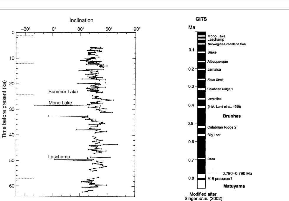
Brunhes and Matuyama Chrons has increased in the last 4 years (Fig-

ure G19). Lund et al. (1998) reported 14 such events in the Brunhes

Chron. Merrill and McFadden (1994) questioned such a large number

of polarity changes, since it would imply that the reversed polarity

state was substantially less stable than the normal state during the

Brunhes Chron, whereas the dynamo equations show that the two

polarities must be statistically the same.

Singer et al. (1999) later identified new short-lived polarity events

between 1.18 and 0.78 Ma and suggested that during this period of

the Matuyama reversed chron there were at least 7, and perhaps more

than 11, attempts by the geodynamo to reverse, implying that the geo-

dynamo was equally unstable in this part of the Matuyama Chron as it

was in the Brunhes Chron. This was confirmed by Channell et al.

(2002) who reported four subchrons and seven excursions in the

Matuyama Chron.

The large number of subchrons and excursions in the Brunhes and

Matuyama Chrons raises a number of unanswered questions on the

stability of the Earth’s magnetic field. One problem is the lack of

reversals observed over geologic time—the oldest known reversal

occurred 3500 Ma ago. There is fair coverage for the last 1 Ma,

but comparatively few records older than 2 Ma. Thus, any conclu-

sions reached about the behavior of the field during the last 2 Ma

may not be true for earlier times. Another problem is dating—we can-

not give accurate ages for events that last only a few thousand years or

less. Possible explanations for excursions are that they are simply the

expression of large amplitude changes in the secular variation, that

they are aborted attempts to reverse, or that they are the result of

chaotic behavior in the nonlinear system of equations that govern the

magnetic field.

An interesting further question is what is the distinction, if any,

between excursions and reversals. A possible explanation for this has

been given by Gubbins (1999) who suggested that the Earth’s inner

core (IC) could stabilize the magnetic field. The IC is solid and

changes in the field can only take place by electrical diffusion. On

the other hand, changes in the field in the outer core (OC) can take

place much faster since they result from convection in the OC which

is fluid. Gubbins proposed that excursions arise when a field reversal

takes place in the OC, but not in the IC. A full reversal only occurs

when the field reversal in the OC persists long enough for the field

in the IC to change polarity as well. If Gubbins’ explanation is correct,

then excursions would be global. It is also consistent with the approx-

imate ratio of excursions to reversals observed in the Brunhes and

Matuyama Chrons.

Jack A. Jacobs

Bibliography

Channell, J.E.T., Mazaud, A., Sullivan, P., Turner, S., and Raymo,

M.E., 2002. Geomagnetic excursions and paleointensities in the

Matuyama Chron at Ocean Drilling Program sites 983 and 984

(Iceland Basin). Journal of Geophysical Research, 107(B6):

doi:10.1029/2001JB000491.

Figure G18 Inclination versus age profile for the

paleomagnetically valid section at Hole 480 from 5 to 62 ka

(5–49 m subbottom). The horizontal dotted segments at the age

ordinate indicate the calibration points for the age estimates: the

top of the section and the oxygen isotope stage boundaries. (After

Levi and Karlin, 1989.)

Figure G19 Geomagnetic instability timescale (GITS) for the

Brunhes Chron (proposed events which require further verification

are labeled with italic letters). Black corresponds to normal

polarity and white to reverse polarity. (After Knudsen et al., 2003.)

312 GEOMAGNETIC EXCURSION

Gubbins, D., 1999. The distinction between geomagnetic excursions

and reversals. Geophysical Journal International, 137:F1–F3.

Knudsen, M.F., Abrahamsen, N., and Riisager, P., 2003. Paleomag-

netic evidence from Cape Verde Islands basalts for fully reversed

excursions in the Brunhes Chron. Earth and Planetary Science

Letters, 206: 199–214.

Levi, S., and Karlin, R., 1989. A sixty thousand year paleomagnetic

record from Gulf of California sediments: secular variation, late

Quaternary excursions and geomagnetic implications. Earth and

Planetary Science Letters, 92: 219–233.

Lund, S.P., Acton, G., Clement, B., Hastedt, M., Okada, M., and

Williams, T., 1998. Geomagnetic field excursions occurred often

during the last million years. EOS Transactions of the American

Geophysical Union, 79: 178–179.

Merrill, R.T., and McFadden, P.L., 1994. Geomagnetic field stability:

reversals and excursions. Earth and Planetary Science Letters,

121:57–69.

Quidelleur, X., Carlut, J., Gillot, P-Y., and Soler, V., 2002. Evolution

of the geomagnetic field prior to the Matuyama-Brunhes transition:

radiometric dating of an 820 ka excursion at La Palma. Geophysi-

cal Journal International, 151:F6–F10.

Singer, B.S., Hoffman, K.A., Chauvin, A., Coe, R.S., and Pringle,

M.S., 1999. Dating transitionally magnetized lavas of the late

Matuyama Chron: toward a new

Ar/

Ar timescale of reversals

and events. Journal of Geophysical Research, 104: 679–693.

Cross-references

Geomagnetic Polarity Reversals

Geomagnetic Secular Variation

Nondipole Field

GEOMAGNETIC FIELD, ASYMMETRIES

The geomagnetic field is produced by dynamo action within the mol-

ten iron in the outer core. This is a dynamic process intimately linked

to cooling of the core and the rapid spin of the Earth. The very nature

of the generative process means that the field is never static but con-

stantly changing, a change referred to as secular variation. Hence, at

any given time, there will be asymmetries in the detail of the field.

Furthermore, in 1934, Cowling showed that a steady poloidal mag-

netic field (the part of the Earth’s field that we see is a poloidal field)

with an axis of symmetry cannot be maintained by motion symmetrical

about that axis. This means that at any given time, the magnetic

field cannot be symmetric about the rotation axis unless the field is

decaying.

The situation is quite different when the field at each point is aver-

aged over a sufficiently long period of time that the statistical varia-

tions of the process are averaged out. The resulting field is known as

the time-average field and, given a symmetric Earth with symmetric

properties, we would expect this time-average field also to be sym-

metric. Indeed, a fundamental assumption used in paleomagnetic

studies is that the time-average field is that of a geocentric axial dipole.

Although an asymmetry in the Earth would not necessarily lead to an

asymmetry in the magnetic field, we expect that any asymmetry in the

time-average geomagnetic field would be a consequence of an asym-

metry in the Earth. Hence, asymmetries in the time-average geomag-

netic field or in the time-average secular variation are of interest

because of the potential to provide information about asymmetries

deep within the Earth. Some aspects of the dynamo process are sensi-

tive to boundary conditions and so any asymmetry is likely to be a

consequence of asymmetry in the boundary conditions on the core.

Hence, the lowermost 150–200 km of the lower mantle, commonly

referred to as the D

layer, probably has the greatest potential to influ-

ence dynamo behavior and produce asymmetries. This is a thermal

chemical boundary layer that exhibits lateral variation in its structure

and composition; analyses of the time-average magnetic field, of the

polarity chronology, of magnetic field reversal paths, and of secular

variation have all been used to examine the impact of these lateral

variations on the magnetic field.

How much time is required to obtain

a time-average field?

The magnetic field of internal origin varies on timescales from less

than a day to more than 10

years. Variations with characteristic times

less than a year are screened out by the semiconducting mantle; the

very long characteristic times are associated with changes in the rate

of magnetic reversals. Most dynamo theorists are of the view that

the characteristic times of dynamo processes are less than 10

years,

and so the changes in the rate of magnetic reversals are usually attrib-

uted to changes in boundary conditions of the outer core.

It is well recognized that under ideal conditions an interval of at

least 10

years is needed to obtain a reasonable estimate of the time-

average field. This reflects the characteristic times of geodynamo pro-

cesses and shows that our record of direct observations is woefully

short to provide a reasonable estimate of the time-average field.

Furthermore, because the magnetic field occasionally experiences

excursions with duration around 10

years, much longer times (more

like 1  10

– 5  10

y) are typically required to obtain a proper

time-average field. Consequently it is necessary to appeal to paleo-

magnetic observations in order to estimate the time-average field.

This then brings with it the problems of inadequate and inaccurate

recording by the rocks and nonuniform distributions in space and

time of the observations. Errors in plate (continent) reconstruction

associated with global tectonics can interfere with magnetic field

reconstruction when time intervals of order 10

y or longer are used

and there is potential for the boundary conditions to have changed

on these longer time frames. Hence, it is difficult to determine the

best time interval to use to estimate the time-average field. Although

paleomagnetists involved in tectonic studies often use shorter time

spans, most investigators examining the time-average magnetic field

properties use a time span around 5  10

The issue is then further complicated by the fact that, on occasion, the

geomagnetic field reverses its polarity, the two states being referred to

as normal (the present state) and reverse polarity. In the past few million

years the average reversal rate has been around 4 to 5 reversals per mil-

lion years and so the field may well have changed polarity several times

during an appropriate averaging interval. If fields of opposite polarity

are simply averaged then the result is likely to be close to zero and quite

unrepresentative of the actual field. In order to avoid this, the normal

and reverse polarity results are either treated separately or combined

by reversing the sign of the reverse polarity data. We do not know

enough about reverse polarity fields to know if it is actually correct to

combine them in this way with normal polarity fields. For example, if

only the dipole component changes sign during a reversal then simply

reversing the sign of the reverse polarity data will invert all of the non-

dipole field when in fact that should not be done. This is unlikely to pro-

duce a false asymmetry in the analysis but there is a minor possibility

that it could incorrectly average out a real asymmetry.

Secular variation asymmetry

In the early 1930s, it was noted that the historical rates of secular var-

iation in the Pacific region were anomalously low. In the 1970s, exten-

sive paleomagnetic investigations of Brunhes-age lava flows from

around the world including, especially, data from the Hawaiian

Islands, showed that the local dispersion of paleodirections of the mag-

netic field were anomalously low for Hawaii. This was interpreted

as being strong evidence for subdued secular variation in the central

Pacific for the past 0.7 Ma, indicating that this was a feature of the

time-average field and not just the historical field. The evidence

GEOMAGNETIC FIELD, ASYMMETRIES 313

seemed reasonably robust because Hawaii was the most extensively

sampled region at that time. Several mechanisms have been suggested,

generally invoking lateral or radial inhomogeneity in D

that sup-

presses the generation, beneath the Pacific, of nondipole fluctuations.

This was interpreted as meaning that the observed variations came

from the dipole field, leading to this region being referred to as the

Pacific dipole window or the Pacific nondipole low.

The claimed low from paleomagnetic evidence has not been sus-

tained by subsequent analyses using much larger data sets. Its origin

seems to reflect inadequate time-averaging that occurred because

basalt flows in Hawaii typically erupt in clusters. Examination in the

1990s of historical data found an intense focus of the nondipole field

in the north Pacific in the 17th century, suggesting that the mere

absence of nondipole field and its secular variation in the Pacific is

only a recent and therefore transient phenomenon. Nevertheless, Con-

stable and Johnson (1999) proposed there still is evidence for some

longitudinal asymmetry in the paleomagnetically estimated secular

variation. If these results are confirmed by more data and subsequent

analyses, it would indicate an asymmetry that is evidenced in the secu-

lar variation data but not in the mean field data.

Polarity asym metries

Over the years, there have been studies that have concluded that the

normal and reverse polarity fields differ in respects other than a simple

change of sign. The questions to be addressed are: is there a bias

toward one or other of the polarities; do the two polarity states have

the same stability; and is the intensity of the field the same for the

two polarity states?

The equations governing the geodynamo are complex and nonlinear,

making it extraordinarily difficult to obtain a solution. However, the

equations are even in H, the magnetic field. That is, the equations

are insensitive to the sign of H, and so if H is a solution then so also

is –H. Hence it is to be expected that the two polarities would have the

same statistical properties and any asymmetry would have to be a

consequence of some boundary condition.

Polarity bias

Over the years an enormous amount of effort has been put in to deter-

mine a reliable chronology for reversals as far back as possible. Such a

chronology is now quite well determined for the past 170 Ma from

analyses of marine magnetic anomalies. As the reversal timescale

developed it became clear that the character of the reversal pattern

has changed markedly with time. The most obvious change occurred

about 118 Ma ago, when the field apparently locked in to a normal

polarity state and remained that way for the next 35 Ma, after which

reversals again occurred. Similarly, during the late Paleozoic the field

was locked in to a single polarity. This phenomenon of long intervals

of time with a single polarity (known as superchrons) has been inter-

preted as the field exhibiting a clear preference for one polarity state

over the other and has been referred to as polarity bias. It is interesting

to note that during the late Paleozoic this apparent bias was for reverse

polarity but during the Cretaceous it was for normal polarity, suggest-

ing that the (interpreted) bias has been a function of time. This per-

ceived polarity bias was attributed to boundary conditions imposed

by the D

layer. Improved data and a better understanding of the rever-

sal process suggest a more simple interpretation. The process produ-

cing reversals was evolving in such a way that the reversal rate

gradually decreased from about 165 Ma until at about 118 Ma the rate

became zero. At that stage, the field was locked in to whatever polarity

it had at the time. Some time later the evolution of the process changed

and at about 83 Ma reversals again started occurring, the rate gradually

increasing from then until the present. Hence, superchrons represent a

time when the reversal process ceased rather than representing a time

of preference for one polarity state over the other. As such, they do

not represent an asymmetry.

Relative stabilities of the two polarity states

Excluding superchrons, when the reversal process was in abeyance,

the intervals of time between reversals may be modeled as a gamma

distribution. This distribution depends on two parameters: the rate at

which the reversals occur; and a parameter k that describes the shape

of the distribution. If the gamma parameter, k, equals 1 then the pro-

cess is the simple Poisson process and the occurrence of an event

(reversal) has no impact on the probability of a future event; the pro-

cess has no memory. For k > 1 the probability of a future reversal

drops to zero as soon as a reversal occurs and then gradually recovers

to its undisturbed value. Thus, the process has a memory of the

previous event and this memory temporarily depresses the probability

of occurrence of future events. Hence, the parameter k can be inter-

preted in terms of the stability of the field (against a further reversal)

immediately after a reversal. Early studies suggested that k is different

for the two polarities, indicating that the relative stabilities of the

polarity states are different. A concern with these early studies was that

the sense of this asymmetry was sensitive to minor details in the polar-

ity chronology. A major problem is that it is easy to miss a short inter-

val in the polarity record, and this has major consequences for

interpretation. Consider the situation if a short reverse interval is

missed. The three-interval polarity segment normal-reverse-normal

appears as a single-interval-normal polarity segment: the three original

intervals have been incorrectly concatenated into a single interval. It is

simple to show that if three intervals are drawn at random from a Pois-

son distribution (k ¼ 1) and concatenated into a single interval, then

the result is the same as drawing a random interval from a gamma

distribution with k ¼ 3. Hence, when short intervals are missed it erro-

neously increases the estimated value of k, and this was not appre-

ciated in the early studies. With this in mind, and with improved

data, it is now apparent that the data are consistent with the two pola-

rities having the same value of k. Indeed, for the reversal process, k is

close to 1 and so the process is nearly Poisson, if not actually Poisson.

Intensity of the field

Reliable determination of the paleointensity of the geomagnetic field is

notoriously difficult. Consequently, conclusions based on paleointensi-

ties are generally less robust than those based on paleodirections or on

the reversal chronology. Nevertheless, paleointensities are an impor-

tant source of information. During the 1980s several studies indica ted

that there were minor but statistically significant differences in the dis-

tributions of paleointensity for the normal and reverse polarity fields.

However, none of these observations was robust and each suffered

from structural problems such as dependence on one or two extreme

values or poor spatial distribution of observations. Further work has

not supported these apparent differences and there now seems no

reason to reject the simple view that the two polarity states have a

common time-average paleointensity.

Structure of the normal and reverse polarity fields

By far the most common way to analyze the geomagnetic field is

through the use of spherical harmonics. The lower-degree harmonics

are probably best known by the terms dipole (degree 2), quadrupole

(degree 3), and octupole (degree 4). Zonal harmonics are harmonics

that are symmetrical about the spin axis and dominate the structure

of the time-average field. In the late 1970s and into the 1980s, analyses

of data from the past 5 Ma indicated that the structure of the time-

average reverse polarity field has been discernibly different from that

of the time-average normal polarity field. Specifically, it appeared

that the time-average reverse polarity field had a proportionately larger

quadrupole and octupole content than the time-average normal polarity

field. However, there were (and remain) significant problems with the

data. The data came primarily from lava flows on continents and islands

and from deep-sea sedimentary cores, which generally provided only

values of the paleomagnetic inclination. The spatial distribution of the

314 GEOMAGNETIC FIELD, ASYMMETRIES

data is poor, particularly in the southern hemisphere, and the data are

poorly distributed in time. Also, rock magnetic and other effects can

produce spurious estimates of odd-degree harmonics, particularly the

octupole term. Later work has shown that these early conclusions were

not robust and were mainly due to data artifacts.

Polarity trans ition asymmetry

Our understanding of the structure of the field during transition from

one polarity to the other is, at best, rudimentary. Despite the fact that

the field at the Earth’s surface is unlikely to be dominantly dipolar dur-

ing a transition, it is standard practice to use the field direction to

calculate the position on the Earth’s surface where the pole would be

if the field were dipolar. This is referred to as a virtual geomagnetic

pole, or VGP. In the absence of a dominant dipolar field structure it

would be expected that, for a single reversal transition, the VGP tran-

sition path would be quite different for observations taken from differ-

ent locations. Of particular interest here is the fact that in the absence

of a persistent asymmetry in the Earth, there should be no consistency

in the VGP transition paths from one reversal transition to another.

Several investigators have noted the existence of apparently pre-

ferred VGP polarity transition paths, both within individual transitions

and persisting across several different transitions. Indeed, there is also

some suggestion of similar preferential paths in VGP movement as a

consequence of normal secular variation. There are also proponents

for periods of VGP stasis during transitions with preferred positions

for the clustering of VGPs. Appeals have been made to the existence

of persistent regions of relatively high electrical conductivity in D

anomalous regions of heat flux through D

, or topography at the

core-mantle boundary to influence the dynamo behavior and produce

these preferred paths. Conversely, there are investigators who feel

the interpretation of preferred paths is a consequence of grossly in-

adequate data. This is currently one of the more controversial topics

in paleomagnetism.

Structure of the time-ave rage field

Over the years, several attempts have been made to determine the

structure of the time-average field by undertaking spherical harmonic

analyses of paleomagnetic data for the past 5 Ma. Of particular interest

here is the question of whether any nonzonal harmonic terms are gen-

uinely present in the time-average field. Most of the modelers who

have undertaken these investigations do claim the presence of nonzo-

nal terms, but the agreement between different models is poor and this

suggests that the conclusions are as yet not robust. As already dis-

cussed, there is no reliable evidence for polarity asymmetry and so a

comparison of normal and reverse polarity results can be used to

assess errors in the estimation of individual harmonic terms. Such a

comparison suggests that the actual errors exceed the formal errors

assigned by modelers.

Once again there are questions regarding reliability of the data. The

data are not well distributed either in space or in time, and it is difficult

to detect small rotations in the rocks providing the data. Consequently,

our knowledge about the structure of the time-average field remains

inconclusive and there is inadequate robust evidence to identify any

specific asymmetries.

Field structure from direct observations

Spherical harmonic models have been created using data from mag-

netic observatories, satellites, and (corrected) ancient mariner logs.

There are now models based on these data that extend from approxi-

mately 400 years ago to the present. While this time span is well short

of that required to obtain a valid time-average magnetic field, some of

the results combined with theory have stimulated research on possible

long-term magnetic field asymmetry.

In particular, Jeremy Bloxham and David Gubbins found four lobes

(in two pairs) in the structure of the field that are placed approximately

symmetrically on either side of the equator at 60



latitude and at

120



W and 120



E longitude. Most of the nondipole field drifts west-

ward, but these flux lobes appear to have been fixed for the time inter-

val investigated. A third north-south pair of lobes is required to

produce symmetry, and the speculation is that such a third pair

has been disrupted by fluid flow near the surface of the outer core.

Bloxham and Gubbins hypothesized that the stationary lobes reflect

convection rolls found much earlier in weak-field dynamo models by

Fritz Busse. (“Weak-field” means that the magnetic field has a negligi-

ble effect on fluid motions in the core. Most theory today involves

strong-field models.) However, dynamo models indicate that the con-

vection rolls should drift westward or eastward depending on the

details of the model. Thus, it was posited that there are thermal anoma-

lies that pin the flux lobes to certain locations in the lowermost mantle.

If true, this would lead to long-term asymmetry in the time-average

magnetic field. Gubbins and Bloxham also emphasize that the data

show a persistent low secular variation in the Pacific hemisphere

and, as already discussed, this would also lead to a manifestation of

asymmetry in the secular variation data.

Conclusion

Dynamo theory is notoriously complex and even with the computing

power available today a working model, based on parameters that actu-

ally match those in the Earth, remains elusive. Hence, it is not currently

possible to predict that the particular asymmetry in the Earth will man-

ifest as a particular asymmetry in the geomagnetic field. Thus, although

there are several mechanisms that it is speculated might lead to geomag-

netic asymmetry, such as anisotropy in the inner core, asymmetry in any

initial field, thermal-electric and battery effects originating in the man-

tle, or thermal and chemical heterogeneities in D

, there is no robust

evidence that this would actually occur. Certainly, it is not currently

possible to invert from an observed asymmetry in the geomagnetic field

to the underlying cause of that asymmetry. However, dynamo models do

indicate that thermal structure at the base of a mantle does influence the

structure of the field generated by the geodynamo.

The case for or against time-average asymmetry in the magnetic

field and/or its secular variation remains inconclusive. The case against

asymmetry is simple to state: all evidence put forth to advocate asymme-

try contains errors, inadequacies, or debatable assumptions. The case for

asymmetry is more subtle. Proponents recognize the problems, but point

to a variety of data types that each weakly suggest a common location

for an asymmetry of some form in the lowermost mantle. For example,

the stationary flux lobes evidenced in the direct observations, claimed

biases of VGP polarity transition data, and some secular variation data,

have all been used to argue for anomalous mantle near the eastern mar-

gin of the Pacific hemisphere. This is also a region that appears to exhi-

bit different seismic properties. Although a scientific cliché, we

conclude that more data and analyses are required.

Acknowledgments

This article is published with the permission of the Chief Executive

Officer, Geoscience Australia.

Phillip L. McFadden and Ronald T. Merrill

Bibliography

Bloxham, J., and Gubbins, D., 1985. The secular variation of the

Earth’s magnetic field. Nature, 317: 777–781.

Bloxham, J., and Gubbins, D., 1986. Geomagnetic field analysis. IV.

Testing the frozen-flux hypothesis. Geophysical Journal of the

Royal Astronomical Society, 84: 139–152.

Constable, C., and Johnson, C., 1999. Anisotropic paleosecular varia-

tion models: implications for geomagnetic field observables. Phy-

sics of the Earth and Planetary Interiors, 115:35–51.

GEOMAGNETIC FIELD, ASYMMETRIES 315