Gubbins D., Herrero-Bervera E. Encyclopedia of Geomagnetism and Paleomagnetism

Подождите немного. Документ загружается.

Similarly, the P

ð mÞ

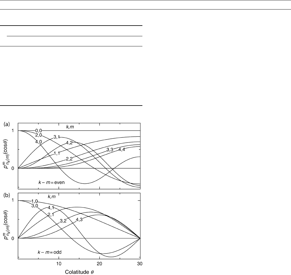
ðcos y Þ, for k  m ¼ odd, are analogous to the sine

functions sinð n yÞ ,0 y  p, in that each is zero at the upper bound-

ary. Here, of course, P

ðmÞ

ð cos yÞ must be nonzero at y ¼ 0 when

m ¼ 0(Figure H9b ). So an expansion over the spherical cap using

ðmÞ

ð cos yÞ , k  m ¼ odd, as basis functions is analogous to an

expansion in Cartesian coordinates using sinð n yÞ as basis functions.

Finding the Legendre functions with zero slope (Eq. (2)) or zero

value (Eq. (3)) at the boundary of the expansion region is therefore

analogous to finding the Fourier cosine and sine basis functions (on

the interval ½0 ; p ) applicable to a given expansion region in Cartesi an

coordinates. Those with zero slope at the boundary are able to fit non-

zero functions there, while those that are zero at the boundary are only

able to fit functions that go to zero there. Of course, we are considering

Eq. (1) to be uniformly convergent, not merely convergent in mean

square (or “ in the mean ”). So to fit an arbitrary function over the

region, one only needs to include the basis functions with zero slope

at the boundary (like the cosine functions). On the other hand, if one

wishes to fit the derivative of the arbitrary function, these basis func-

tions would not do (unless that arbitrary function has zero slope at

the boundary). However, the basis functions that are zero (and whose

derivatives are therefore not zero) at the boundary, will be able to fit

uniformly the derivative of that arbitrary function. Including basis

functions both with zero slope and zero function at the boundary thus

permits the uniform expansion of functions with both arbitrary values

and arbitrar y derivatives at the boundary of the expansion region.

The Legendre functions thus defined comprise two sets of sepa-

rately orthogonal functions, with respect to the weight function siny.

That is, P

ðmÞ

ð cos y Þ and P

ðmÞ

ð cos y Þ are orthogonal when j 6¼ k

and when j  m and k  m are either both odd or both even. However,

they are not orthogonal when j  m ¼ even and k  m ¼ odd (or vice

versa).

The vector magnetic field B

The vector magnetic field B is given by the negative gradient of

Eq. (1). That is, we compute the vertical and the horizontal spheri cal

cap north and east components of B by differentiating Eq. (1) with

respect to the spherical cap coordinates r, y , and l , respect ively (with

appropriate signs and of course including the metrical coefficients 1, r,

and rsiny). Note that only when the spherical cap pole is the

geographic North Pole, are these components the usual geogra phic

components.

We can see now why we need the spherical cap basis functions with

k  m ¼ odd. It is because the north component of the field involves a

differentiation with respect to y. If the north component of the data

happened to be nonzero at y ¼ y

, the north component of the model

would not be uniformly convergent if only basis functions with

dPðcosy

Þ= dy ¼ 0 were included in the model. Of course, if the north

component is not being modeled, the second set of basis functions are

not strictly required (the vertical anomaly field from Magsat data, e.g.,

was modeled by Haines, 1985b). In this case, the constraint on the

derivative of P results in the field having zero slope, with respect to

y, at the cap boundary.

Even if one did not need to fit a derivative, it can still be an advan-

tage to include basis functions that allow for a nonzero derivative at

the boundary of the analysis region. That advantage is in faster conver-

gence (a smaller number of coefficients for a given truncation error),

as discussed by Haines (1990).

Mean square and cross product values for the internal and external

harmonics of the vector field B have been derived by Lowes (1999),

in terms of the harmonics of the potential, as well as for their horizon-

tal and radial components. Power spectra have been defined and

expressed by Haines (1991), and the relationship of spherical cap

harmonics to ordinary spherical harmonics has been described by

De Santis et al. (1999).

Subtraction of a reference field

The price paid for having uniform convergence over a spherical cap by

including both sets of basis functions is that some of these functions

are mutually nonorthogonal. Although most are mutually orthogonal

(those within each of the two sets and all those of different order by

virtue of the orthogonality of the longitude functions), even this sparse

nonorthogonality can have an adverse effect on the coefficient solu-

tion, particularly at high truncation levels. This is because the non-

orthogonality results in an ill-conditioned least-squares matrix, which

will have some nondiagonal terms. The smaller the computer word

size and the larger the field values being fitted, the more serious is this

problem. It is therefore advantageous to subtract a spherical harmonic

reference field from the data, do the spherical cap harmonic fit on the

resulting residuals, and simply add the reference field back on when

Figure H9 Legendre functions P

ðmÞ

ðcos yÞ of nonintegral degree

ð m Þ (given in Table H3) and integral order m , up to index

k ¼ 4: (a) those that have zero slope at the cap boundary

¼ 30



, and (b) those that are zero at the cap boundary.

Table H3 n

(m) for y

= 30˚

k 012345678

0 0.00

1 4.08 3.12

2 6.84 6.84 5.49

3 10.04 9.71 9.37 7.75

4 12.91 12.91 12.37 11.81 9.96

5 16.02 15.82 15.62 14.92 14.18 12.13

6 18.94 18.94 18.58 18.22 17.39 16.50 14.29

7 22.02 21.87 21.72 21.25 20.76 19.81 18.80 16.42

8 24.95 24.95 24.69 24.42 23.84 23.24 22.19 21.07 18.55

396 HARMONICS, SPHERICAL CAP

the full field is required. Which particular harmonic reference field is

used for this purpose is unimportant; the idea is simply to have smaller

numbers in the modeling process so as not to lose too much numerical

accuracy for the given computer word size.

A second difficulty with spherical cap and other regional models, is

the accumulation of errors in upward or downward continuation of the

field (see Upward and downward continuation). The field at the con-

tinuation point, of course depends on field values outside the cap, as

well as inside, and so unless the effect of these outside values could

somehow be compensated for by more complicated boundary condi-

tions, there will be an error in continuing a model based only on field

values inside the cap. Here again, we can get considerable relief from

subtraction of global reference fields, which are models of data from

the whole Earth. Haines (1985a, Figures 3–6) shows the kinds of errors

to expect in upward continuing fields to 300 and 600 km, and the lower

errors when subtracting an International Geomagnetic Reference Field

(IGRF) (q.v.) prior to analysis.

General field s over a cap surface

Previously, we have discussed fitting a harmonic function in a three-

dimensional region of space over a spherical cap, as portrayed in

Figure H8. However, the spherical cap basis functions can also be used

to expand a general function over a (two-dimensional) spherical cap

surface (y  y

; r ¼ r

). That is, there is no constraint for this surface

field to be harmonic since the radial field is not being defined; it can

represent, on the surface, fields that are very complex in three-dimen-

sional space. This is analogous to the expansion theorem for the whole

sphere (e.g., Courant and Hilbert, 1953, Chapter VII, Section 5.3).

The vertical field is able to play the role of the general function by

considering only the internal field (i.e., putting K

¼ 0), and setting

r ¼ a. The factor ½n

ðmÞþ1 arising from the differentiation with

respect to r can also be set to unity. Similarly, the north and east com-

ponents can be made to play the role of north and east derivatives of

a general function by similar modifications (see Haines, 1988, p. 422

for details). This latter aspect can be used to model electric fields

(horizontal derivatives of an electric potential) over a surface in

the ionosphere. Although an electric potential satisfies Poisson’s equa-

tion in three-d imensional space, it can be treated as a general function

on the spherical surface.

This surface expansion is in fact the solution of the two-dimensional

eigenvalue problem in the two variables (colatitude and longitude)

whose functions (Legendre and trigonometric) were orthogonalized

in the solution of the three-dimensional differential equation. This is

a common technique in expansion methods. In Cartesian coordinates,

for example, the solution to Laplace’s equation in three-dimensional

space (“Rectangular Harmonics”) gives rise to a surface expansion

(two-dimensional “Fourier Series”) simply by finding the eigensolu-

tions in the coordinates whose (trigonometric) functions were orthogo-

nalized there. Again, these Fourier series allow the expansion of a very

large class of functions, certainly functions that are in no way con-

strained as are the rectangular harmonic functions of three-dimensional

space. Of course, we can go down another dimension and expand one-

dimensional functions in either of the surface variables. This gives an

expansion, on the spherical cap, in trigonometric functions for longi-

tude and in Legendre functions for colatitude, analogously to the

one-dimensional trigonometric Fourier series in Cartesian coordinates.

Example application

Regional magnetic field models over Canada have been produced

every 5 years since 1985 using spherical cap harmonics. For each

model, the IGRF at an appropriate epoch is subtracted from the data,

and a spherical cap harmonic model of the residuals is then deter-

mined. (This also provides an estimate of the “error” or wavelength

limitations of the IGRF that was subtracted.) The final model, obtained

by adding the IGRF back on to the spherical cap model, is referred to

as the Canadian Geomagnetic Reference Field (CGRF). Details of the

data and processing methods used for the 1995 CGRF have been given

by Haines and Newitt (1997).

G.V. Haines

Bibliography

Chapman, S., and Bartels, J., 1940. Geomagnetism, Vol. II. New York:

Oxford University Press.

Courant, R. and Hilbert, D., 1953. Methods of Mathematical Physics,

translated and revised from the German original, Vol. I. New York:

Interscience Publishers.

Davis, H.F., 1963. Fourier Series and Orthogonal Functions. Boston:

Allyn and Bacon.

De Santis, A., Torta, J.M., and Lowes, F.J., 1999. Spherical cap har-

monics revisited and their relationship to ordinary spherical harmo-

nics. Physics and Chemistry of the Earth (A), 24: 935–941.

Haines, G.V., 1985a. Spherical cap harmonic analysis. Journal of Geo-

physical Research, 90: 2583–2591.

Haines, G.V., 1985b. Magsat vertical field anomalies above 40



from spherical cap harmonic analysis. Journal of Geophysical

Research, 90: 2593–2598.

Haines, G.V., 1988. Computer programs for spherical cap harmonic

analysis of potential and general fields. Computers and Geos-

ciences, 14: 413–447.

Haines, G.V., 1990. Modelling by series expansions: a discussion.

Journal of Geomagnetism and Geoelectricity, 42: 1037–1049.

Haines, G.V., 1991. Power spectra of subperiodic functions. Physics of

the Earth and Planetary Interiors, 65: 231–247.

Haines, G.V., and Newitt, L.R., 1997. The Canadian Geomagnetic

Reference Field 1995. Journal of Geomagnetism and Geoelectri-

city, 49: 317–336.

Lowes, F.J., 1999. Orthogonality and mean squares of the vector fields

given by spherical cap harmonic potentials. Geophysical Journal

International, 136: 781–783.

Smythe, W.R., 1950. Static and Dynamic Electricity, 2nd ed. New

York: McGraw-Hill.

Cross-references

Harmonics, Spherical

IGRF, International Geomagnetic Reference Field

Upward and Downward Continuation

HARTMANN, GEORG (1489–1564)

Hartmann was born on February 9, 1489, at Eggolsheim, Germany.

After studying theology and mathematics at Cologne around 1510,

he spent some time in Rome, where he ranked Andreas, the brother

of Nicholas Copernicus, amongst his friends. Hartmann belonged to

that class of Renaissance scholar who, while the recipient of a learned

education, also had a fascination with mechanics, horology, instrumen-

tation, and natural phenomena. His principal claim to fame as a student

of magnetism lay in his discovery that in addition to the compass nee-

dle pointing north, it also had a dip, or inclination, out of the horizon-

tal. He claims to have noticed, for instance, that in Rome, the needle of

a magnetic compass dipped by 6



towards the north. Although his

numerical quantification of this phenomenon was wrong, the compass

does, indeed, dip in Rome, as it does in most nonequatorial locations.

Although Hartmann never published his discovery, he did commu-

nicate it in a letter of 4 March 1544 to Duke Albert of Prussia. Unfor-

tunately, this remained unknown to the wider world for almost the next

three centuries, until it was finally printed in 1831. Hence, Hartmann’s

discovery had no influence on other early magnetical researchers, and

credit for the discovery of the “dip” went to the Englishman Robert

HARTMANN, GEORG (1489–1564) 397

Norman (q.v.), who published his own independent discovery in A

Newe Attractive (London, 1581).

Hartmann was a priest by vocation, and held several important ben-

efices. He settled in Nuremberg in 1518, where he was no doubt in his

element, as that city was one of Europe’s great centers for the manu-

facture of clocks, watches, instruments, ingenious firearms, and other

precision metal objects. He collected astronomical and scientific

manuscripts and was associated with the Nuremberg observational

astronomer Johann Schöner, as well as Joachim Rheticus, who saw

Copernicus’ De Revolutionibus through the press at Nuremberg in

1543. Hartmann died in Nuremberg on April 9, 1564.

Allan Chapman

Bibliography

Heger, K., 1924. Georg Hartmann von Eggolsheim. Der Fränkische

Schatzgräber 2:25–29.

Hellmann, G. (ed.), Rara Magnetica 1269–1599, Neudrucke von

Schriften und Karten über Meteorologie und Erdmagnetismus

no. 10 (Berlin, 1898). Reprints Hartmann’s letter to Duke Albert of

Prussia. Letter first noticed in Prussian Royal Archives, Königsberg;

see J. Voigt, in Raumer ’s Historisches Taschenbuch II (Leipzig,

1831), 253–366.

Ritvo, L.B., ‘Georg Hartmann’, Dictionary of Scientific Biography

(Scribner’s, New York, 1972–).

Zinner, Ernst, Deutsche und niederländische astronomische Instrumente

des 11–18 Jahrhunderts (Munich, 1956).

HELIOSEISMOLOGY

Helioseismology is the study of the interior of the Sun using observa-

tions of waves on the Sun’s surface. It was discovered in the 1960s

by Leighton, Noyes, and Simon that patches of the Sun’s surface

were oscillating with a period of about 5 min. Initially these were

thought to be a manifestation of convective motions, but by

the 1970s it was understood from theoretical works by Ulrich and

Leibacher and Stein and from further observational work by Deubner

that the observed motions are the superposition of many global reso-

nant modes of oscillation of the Sun (e.g., Deubner and Gough,

1984, Christensen-Dalsgaard, 2002). The Sun is a gaseous sphere,

generating heat through nuclear fusion reactions in its central region

(the core) and held together by self-gravity. It can support various

wave motions, notably acoustic waves and gravitational waves; these

set up global resonant modes. The modes in which the Sun is observed

to oscillate are predominantly acoustic modes, though the acoustic

wave propagation is modified by gravity and the Sun’s internal strati-

fication, and by bulk motions and magnetic fields. The observed prop-

erties of the oscillations, especially their frequencies, can be used to

make inferences about the physical state of the solar interior. The exci-

tation mechanism is generally believed to be turbulent convective

motions in subsurface layers of the Sun, which generate acoustic noise.

This is a broadband source, but only those waves that satisfy the

appropriate resonance conditions constructively interfere to give rise

to resonant modes.

There are many reasons to study the Sun. It is our closest star and

the only one that can be observed in great detail, so it provides an

important input to our understanding of stellar structure and evolution.

The Sun greatly influences the Earth and near-Earth environment, par-

ticularly through its outputs of radiation and particles, so studying it is

important for understanding solar-terrestrial relations. And the Sun

also provides a unique laboratory for studying some fundamental

physical processes in conditions that cannot be realized on Earth.

From the 1980s up to the present day, much progress has been made

in helioseismology through analysis of the Sun’s global modes of

oscillation. Some of the results, on the Sun’s internal structure and

its rotation, are given below. Though not discussed here, similar stu-

dies are now also beginning to be made in more limited fashion for

some other stars, in a field known as asteroseismology. In the past dec-

ade, global mode studies of the Sun have been complemented by so-

called local helioseismology, techniques such as tomography which

have been used to study flows in the near-surface layers and flows

and structures under sunspots and active regions of sunspot com-

plexes. Local helioseismology is also discussed below.

Solar oscill ations

The Sun’s oscillations are observed in line-of-sight Doppler velocity

measurements of the visible solar disk, and in measurements of varia-

tions of the continuum intensity of radiation from the surface. The

latter are caused by compression of the radiating gas by the waves.

Spatially resolved measurements are obtained by observing separately

different portions of the visible solar disk; but the motions with the lar-

gest horizontal scales are also detectable in observations of the Sun as

a star, in which light from the whole disk is collected and analyzed as a

single time series. To measure the frequencies very precisely, long,

uninterrupted series of observations are desirable. Hence, observations

are made from networks of dedicated small solar telescopes distributed

in longitude around the Earth (networks such as the Global Oscillation

Network Group [GONG] making 1024  1024-pixel resolved obser-

vations and the Birmingham Solar Oscillation Network [BiSON]

making Sun-as-a-star observations) or from space (for instance, the

Solar and Heliospheric Orbiter [SOHO] satellite has three dedicated

helioseismology instruments onboard, in decreasing order of resolution

MDI, VIRGO and GOLF). In Doppler velocity, the amplitudes of indi-

vidual modes are of order 10 cm s

1

or smaller, their superposition

giving a total oscillatory signal of the order of a few kilometers per

second. The highest amplitude modes have frequencies n of around

3mHz.

The outer 30% of the Sun comprises a convectively unstable region

called the convection zone (e.g., Christensen-Dalsgaard et al., 1996).

The solar oscillations are stochastically excited by turbulent convec-

tion in the upper part of the convection zone. The modes are both

excited and damped by their interactions with the convection.

Although large excitation events such as solar flares may occasionally

contribute, the dominant excitation is probably much smaller-scale and

probably takes place in downward plumes where material previously

brought to the surface by convection has cooled and flows back into

the solar interior. These form a very frequent and widespread set of

small-scale excitation sources.

The fluid dynamics of the solar interior is described by the fluid

dynamical momentum equation and continuity equation, an energy

equation and Poisson’s equation for the gravitational potential. On

the timescales of the solar oscillations of interest here, the bulk of

the solar interior can be considered to be in thermal equilibrium

and providing a static large-scale equilibrium background state in

which the waves propagate. Treating the departures from the time-

independent equilibrium state as small perturbations with harmonic

time dependence expðiotÞ, where o  2pn is an (as yet) unknown

resonant angular frequency, t is time and i ¼

ﬃﬃﬃﬃﬃﬃﬃ

1

, the above mentioned

equations can be linearized in perturbation quantities and constitute

a coupled set of linear equations describing the waves. The time-

scales of the solar oscillations are sufficiently short that the energy

equation can be replaced by the condition that the perturbations

of pressure ( p) and density ðrÞ are related by an adiabatic relation.

At high frequencies, pressure forces provide the dominant restoring

force for the perturbed motions, giving rise to acoustic waves. A

key quantity for such acoustic waves is the adiabatic sound speed

c, which varies with position inside the Sun: c

¼ G

p=r, where

is the first adiabatic exponent (G

¼ 5=3 for a perfect mona-

tomic gas). To an excellent approximation, p / rT =m, where T is

temperature and m is the mean molecular weight of the gas, so

398 HELIOSEISMOLOGY

c / T

1=2

inside the Sun. Except for wave propagating exactly ver-

tically, inward-propagating waves get refracted back to the surface

at some depth, because the temperature and hence sound speed

increase with depth. Near the surface, outward-propagating waves

also get deflected, by the sharply changing stratification in the

near-surface layers. Hence the acoustic waves get trapped in a reso-

nant cavity and form modes, with discrete frequencies o.Toa

good approximation, the Sun’s structure is spherically symmetric,

hence, the horizontal structure of the eigenfunctions of the modes

is given by spherical harmonics Y

, where integers lðl  0 Þ and

mðl  m  lÞ are respectively called the degree and azimuthal

order of the mode. The structure of the eigenfunction in the radial

direction into the Sun is described by a third quantum number n,

called the order of the mode: the absolute value of n is essentially

the number of nodes in the (say) pressure perturbation eigenfunc-

tion between the center and the surface of the Sun. Hence, each

resonant frequency can be labeled with three quantum numbers

thus: o

nlm

. The labeling is such that at fixed l and m, the frequency

nlm

is a monotonic increasing function of n.

In a wholly spherically symmetrical situation the frequencies would

be independent of m. However, the Sun’s rotation, as well as any other

large-scale motions, thermal asphericities, and magnetic fields break

this degeneracy and introduce a dependence on m in the eigenfrequen-

cies. The modes of different m but with the same values of n and l are

called a multiplet: it is convenient also to introduce the mean multiplet

frequency o

High-frequency modes, with positive values of the order n, are

essentially acoustic modes (p modes): for them, the dominant restoring

force is pressure. Low-frequency modes, with negative values of n, are

essentially gravity modes (g modes) set up by gravity waves, which

can propagate where there is a stable stratification. There is an inter-

mediate mode with n ¼ 0: this is the so-called fundamental or f mode.

For large values of l, the f mode has the physical character of a surface

gravity mode. The observed global modes of the Sun are p modes and

f modes. Modes of low degree (mostly l ¼ 0; 1; 2; 3) are detectable in

observations of the Sun as a star: low-degree p modes are sensitive to

conditions throughout the Sun, including the energy-generating core.

Spatially resolved observations have detected p and f modes up to

degrees of several thousand: such modes are no longer global in char-

acter, but nonetheless measuring their properties conveys information

about the Sun’s outer subsurface layers. Internal g modes have not

unambiguously been observed to date, and they are expected to have

small amplitudes at the surface: this is because their region of propaga-

tion is the stably stratified radiative interior and they are evanescent

through the intervening convection zone.

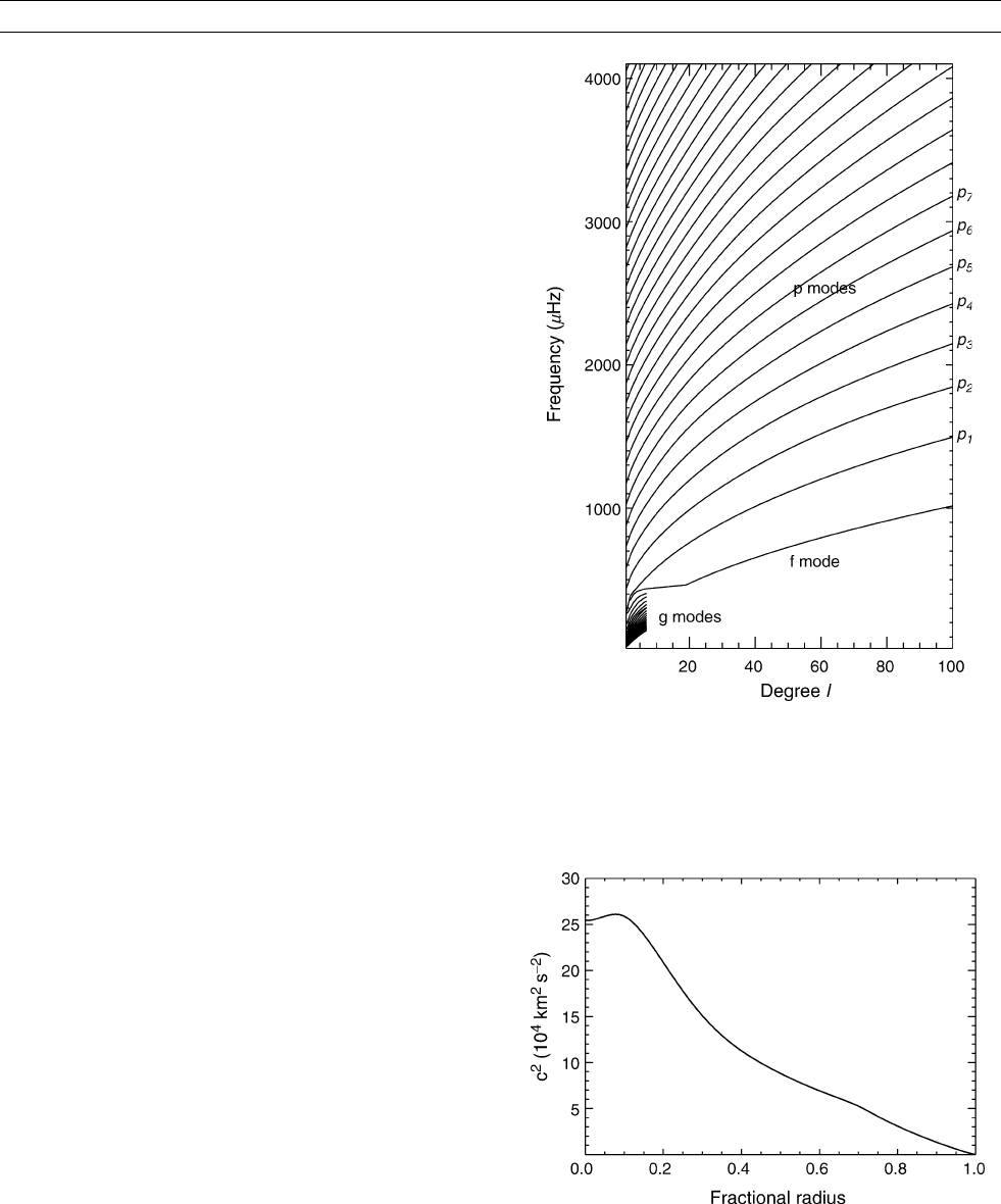
The computed mean multiplet frequencies for modes of a current

model of the Sun are shown in Figure H10. Points on each branch

of the dispersion relation (each corresponding to a single value of n)

have been joined with continuous curves.

Results from global-mode helioseismology

The frequencies of the Sun’s global modes are estimated by making

suitable spatial projections and temporal Fourier transformations of

the observed Doppler or intensity fluctuations. From these, using a

variety of fitting or inversion techniques (similar to those used in other

areas of, e.g., geophysics and astrophysics), properties of the solar

interior can be deduced. Indeed, helioseismology has borrowed and

adapted various approaches and ideas on inversion from geophysics,

notably those of G. Backus and F. Gilbert (Backus and Gilbert,

1968, 1970). One of the principal deductions from helioseismology

has been the sound speed as a function of position in the Sun (e.g.,

Gough et al., 1996). The value of this deduction lies not in the precise

value of the sound speed but in the inferences that follow concerning

the physics that determines the sound speed. The sound speed in a

solar model that is closely in agreement with the helioseismic data is

illustrated in Figure H11. As discussed above, the adiabatic sound

speed c is related to temperature T, mean molecular weight m, and adia-

batic exponent G

by c

/ G

T=m, where the constant of proportional-

ity is the gas constant. The general increase in sound speed with depth

reflects the increase in temperature from the surface to the center of the

Figure H11 Square of the adiabatic sound speed c inside a model

of the present Sun, as a function of fractional radius (center at 0,

photospheric surface at 1.0).

Figure H10 Mean multiplet cyclic frequencies n

ð¼ o

=2pÞ of

p, f, and g modes of a solar model, as a function of the mode

degree l. The low-order p modes are labelled according to the

value of the mode order n. The g modes are only illustrated up to

l ¼ 7 and for jnj20.

HELIOSEISMOLOGY 399

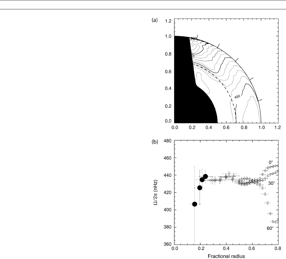
Sun. The gradient of the temperature, and hence of the sound speed, is

related to the physics by which heat is transported from the center to

the surface. In the bulk of the Sun, that transport is by radiation;

but in the outer envelope the transport is by convection. A break in

the second derivative of the sound speed near a fractional radius

of 0.7 indicates the transition between the two regimes and has

enabled helioseismology to determine the location of the base of the

convection zone: this is important because it delineates the region in

which chemical elements observed at the surface are mixed and homo-

genized by convective motions. Beneath the convection zone, the gra-

dients of temperature and sound speed are influenced by the opacity of

the material to radiation: it has thus been possible to use the seismi-

cally determined sound speed to find errors in the theoretical estimates

of the opacity, which is one of the main microphysical inputs for mod-

eling the interiors of stars. Not readily apparent on the scale of

Figure H11 is the spatial variation of G

and hence of sound speed

in the regions of partial ionization of helium and hydrogen in the outer

2% of the Sun. This variation depends on the equation of state of the

material and on the abundances of the elements: it has been used to

determine that the fractional helium abundance by mass in the convec-

tion zone, which is poorly determined from surface spectroscopic

observations, is about 0.25. This is significantly lower than the value

of 0.28 believed from stellar evolutionary models to have been the

initial helium abundance of the Sun when it formed. The deficiency

of helium in the present Sun’s convection zone is now understood to

arise from gravitational settling of helium and heavier elements out

of the convection zone and into the radiative interior over the 4.7 Ba

that the Sun has existed as a star. This inference is confirmed by an

associated slight modification to the sound speed profile beneath the

convection zone.

The dip in the sound speed at the center of the Sun is the signature

of the fusion of hydrogen to helium that has taken place over the Sun’s

lifetime: the presence of helium increases the mean molecular weight

m, decreasing the sound speed. Thus the amount of build-up of helium

in the core is an indicator of the Sun’s age. Apart from inversions, a

sensitive indicator of the sound speed in the core is the difference

 n

n1;lþ2

between frequencies of p modes of low degree

ðl ¼ 0, 1, 2, 3Þ differing by two in their degree. Such pairs of modes

penetrate into the core and have similar frequencies and hence very

similar sensitivity to radial structure in the outer part of the Sun, but

have different sensitivities in the core.

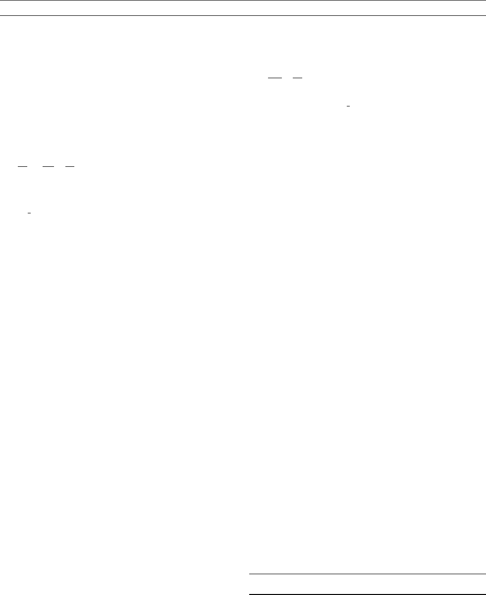
Another major deduction of global-mode helioseismology has been

the rotation as a function of position through much of the solar interior

(Figure H12) (e.g., Thompson et al., 1996, 2003). In the convection

zone, it has been discovered that the rotation varies principally with

latitude and rather little with depth: at low solar latitudes the rotation

is fastest, with a rotation period of about 25 days; while at high lati-

tudes the rotation periods in the convection zone are in excess of 30

days. These rates are consistent with deductions of the surface rotation

from spectroscopic observations and from measurements of motions of

magnetic features such as sunspots. The finding was at variance with

some theoretical expectations that the rotation in the convection zone

would be constant on Taylor columns. At low- and mid-latitudes there

is a near-surface layer of rotational shear, which may account for the

different rotational speeds at which small and large magnetic features

are observed to move. Near the base of the convection zone, the lati-

tudinally differential rotation makes a transition to latitudinally inde-

pendent rotation. This gives rise to a layer of rotational shear at low

and high latitudes, which is called the tachocline. It is widely believed

that the tachocline is where the Sun’s large-scale magnetic field is gen-

erated by dynamo action, leading to the 11-year solar cycle of sunspots

and the large-scale dipole field. Deeper still the rotation appears to be

consistent with solid-body rotation, presumably caused by the pre-

sence of a magnetic field. In the core, there is some hint of a slower

rotation, but the uncertainties on the deductions are quite large: none-

theless, some earlier theoretical predictions that the core would rotate

much faster than the surface, a relic of the Sun’s faster rotation as a

young star, are strongly ruled out by the seismic observations. Super-

imposed on the rotation of the convection zone are weak but coherent

migrating bands of faster and slower rotation (of amplitude only a few

meters per second, compared with the surface equatorial rotation rate

of about 2 km s

1

), which have been called torsional oscillations:

the causal connection between the migrating zonal flows and the sun-

spot active latitudes, which also migrate during the solar cycle, is as

yet uncertain. There have also been reported weak variations, with per-

iodicities around 1.3 years, in the rotation rate in the deep convection

zone and in the vicinity of the tachocline. To date there has been no

direct helioseismic detection of magnetic field in the region of the

tachocline: indeed, because the pressure increases rapidly with depth,

a field there would have to have a strength of order 10

Gauss to have

a significant direct influence on the mode frequencies. Thus detecting

Figure H12 (a) Contour plot of the rotation rate inside the Sun

inferred from MDI data. The rotation axis is up the y-axis, the

solar equator is along the x-axis. Contour spacings are 10 nHz;

contours at 450, 400, and 350 nHz are thicker. The shaded region

indicates where a localized solution has not been possible with

these data. (b) The rotation rate deeper in the interior, on three

radial cuts at solar latitudes 0



; 30



, and 60



, using data from

Sun-as-a-star observations by BiSON and spatially resolved

observations by the LOWL instrument.

400 HELIOSEISMOLOGY

the effect of a temporally varying magnetic field on the angular

momentum may be the most likely way to infer seismically the pre-

sence of such a field in the deep interior. On the other hand, near-

surface magnetic fields can influence mode frequencies in a detectable

way, because the pressure is much lower there; and there is strong evi-

dence that mode frequencies vary over the solar cycle in a manner that

is highly correlated with the temporal and spatial variation of photo-

spheric magnetic field.

Local helioseismology

Analysis of the Sun’s global mode frequencies has provided an

unprecedented look at the interior of a star, but such an approach has

limitations. In particular, the frequencies sense only a longitudinal

average of the internal structure. To make more localized inferences,

the complementary approaches of local helioseismology are used.

One such technique is to analyze the power spectrum of oscillations

as a function of frequency and the two horizontal components of the

wavenumber in localized patches. To obtain good wavenumber resolu-

tion, the patches are usually quite large: square tiles of up to about

2  10

km on the side. The technique is known as ring analysis,

because at fixed frequency the p-mode power lies on near-circular

rings in the horizontal wavenumber plane. By performing inversions

for the depth dependence under each tile, maps with horizontal resolu-

tion similar to the size of the tiles can be obtained of structures and

particularly of flows in the outer few per cent of the solar interior

(e.g., Toomre, 2003). As well as the zonal flows, the meridional (i.e.,

northward and southward) flow components have also been measured.

Beneath the surface, these are generally found to be poleward in both

hemispheres down to the depth at which the ring analyzes lose resolu-

tion: this depth is of order 10

km. However, the analyses indicate that

the flow patterns in the northern but not the southern hemispheres

changed markedly in 1998–2000 as the Sun approached the maximum

of its 11-year magnetic activity cycle.

Other local techniques include time-distance helioseismology and

acoustic holography. So for example, in time-distance helioseismology,

the travel-time of waves between different points on the surface of

the Sun are used to infer wavespeed and flows under the surface (e.

g., Kosovichev, 2003). This can be achieved on much smaller horizon-

tal scales than have yet been achieved by ring analysis, down to just a

few thousand kilometers. Since individual excitation events are rarely

if ever seen, the travel-times are isolated from the measured Doppler

velocities across the solar disk by cross-correlating pairs of points, or

sets of points. Using high-resolution observations such as those from

the MDI instrument onboard SOHO, travel-times can be measured

between many different locations on the solar surface, and with

different spatial separations which in turn provide different depth sen-

sitivities to subsurface conditions. By comparing the measured travel-

times with those of a solar model, inversion techniques similar to those

used in global mode helioseismology have been used to map condi-

tions in the convection zone using travel-time data. In particular, wave-

speed anomalies and flows under sunspots and active regions of strong

magnetic fields on the surface have been mapped. An unexpected find-

ing has been that the wavespeed beneath sunspots (which in such

regions is not just the sound speed but is modified by the magnetic

field) is increased relative to the spot’s surroundings, except in a shal-

low layer of up to 5000km depth where the wavespeed is decreased.

Such studies are providing much-needed constraints on models of sun-

spot structure and theories of their origin, and on models of the emer-

gence of magnetic flux from the solar interior.

Michael J. Thompson

Bibliography

Backus, G. and Gilbert, F., 1968. The resolving power of gross Earth

data. Geophysical Journal, 16: 169–205.

Backus, G. and Gilbert, F., 1970. Uniqueness in the inversion of inac-

curate gross Earth data. Philosophical Transactions of the Royal

Society of London, Series A, 266: 123–192.

Christensen-Dalsgaard, J., 2002. Helioseismology. Reviews of Modern

Physics, 74: 1073–1129.

Christensen-Dalsgaard, J., et al.,1996. The current state of solar mod-

eling. Science, 272: 1286–1292.

Deubner, F.-L., and Gough, D.O., 1984. Helioseismology: oscillations

as a diagnostic of the solar interior. Annual Review of Astronomy

and Astrophysics, 22: 593–619.

Gough, D.O., et al.,1996. The seismic structure of the Sun. Science,

272: 1296–1300.

Kosovichev, A., 2003. Telechronohelioseismology. In Thompson, M.J.,

and Christensen-Dalsgaard, J. (eds.), Stellar Astrophysical Fluid

Dynamics. Cambridge: Cambridge University Press, pp. 279–296.

Thompson, M.J., Christensen-Dalsgaard, J., Miesch, M.S., and

Toomre, J., 2003. The internal rotation of the Sun. Annual Review

on Astronomy and Astrophysics, 41: 599–643.

Thompson, M.J., et al.,1996. Differential rotation and dynamics of the

solar interior. Science, 272: 1300–1305.

Toomre, J., 2003. Bridges between helioseismology and models of

convection zone dynamics. In Thompson, M.J., and Christensen-

Dalsgaard, J., (eds.), Stellar Astrophysical Fluid Dynamics. Cam-

bridge: Cambridge University Press, pp. 299–314.

Cross-references

Dynamo, Solar

Harmonics, Spherical

Magnetic Field of Sun

Proudman-Taylor Theorem

HIGGINS-KENNEDY PARADOX

For the student learning about properties of the Earth’s core it may be

surprising that the core is solid at its center where its temperature is

highest, while it becomes liquid at a distance of about 1220 km from

the center where the temperature is lower. This property is caused

by the dependence of the melting temperature T

on the pressure p.

That the melting temperature T

of nearly all materials increases with

pressure has been a well-known property for a long time and finds its

most simple expression in Lindemann’s law

¼ 2 g 



=k (Eq. 1)

where k is the compressibility along the melting curve T

(p) and g is

the Grüneisen parameter which, in thermodynamics, is defined by

g ¼

: (Eq. 2)

Here, r denotes the density, a is the coefficient of thermal expansion,

and k

are the isothermal and adiabatic compressibilities, while

and c

are the specific heats at constant volume and constant pres-

sure, respectively. The Grüneisen parameter g plays a prominent role

in studies of the thermal state of planetary interiors since it assumes a

value of the order unity for all condensed materials and does not vary

much with pressure or temperature in contrast to the material properties

on the right hand sides of Eq. (2). Using thermodynamic relationships

one finds (see Grüneisen’s parameter for iron and Earth’s core)

g ¼



¼

] ln V

] ln T



(Eq. 3)

HIGGINS-KENNEDY PARADOX 401

which indicates that g describes the negative slope in logarithmic plots

of volume versus temperature under adiabatic compression. The g used

in relationship (1) is not necessarily the thermodynamic one, since the

melting temperature may be influenced by electronic contributions and

other effects which are not taken into account in Eqs. (2) and (3 ). The

simple approximate relationship (1) called Lindemann’s law is far

from a rigorous law in any mathematical sense and is mentioned here

only as an example of many similar “ laws ” that have been derived in

the literature. For a review and a recent paper, see Jacobs (1987) and

Anderson et al. (2003).

The adiabatic temperature gradient is defined by (see Core,

adiabatic gradient)

] T

] p



(Eq. 4)

Here, the isentropic compressibility k

is well determined in

the Earth ’ s core by seismic data, since the relationship k

rð V



Þ holds where V

and V

are the velocities of propagation

of p (compressional)- and s (shear)-waves. The adiabatic temperature

gradient defines a state where the exchange of fluid parcels from differ-

ent radii can be accomplished without gain or loss of energy when dissi-

pative effects such as those connected with viscous friction can be

neglected. When the increase of temperature with pressure is less than

the adiabatic gradient, a stably stratified state is obtained which requires

an input of energy for the exchange of fluid parcels from different radii.

When the temperature increases more strongly by a finite amount e than

the adiabatic gradient, the static state becomes unstable and convection

sets in. In fact, for dimensions as large as those of the core, the amount

e is minute, such that a state of convection corresponds essentially to

an adiabatic temperature distribution. Since convection flows of suffi-

cient strength are needed to generate the geomagnetic field (Busse,

1975) it has always been assumed that the temperature field of the liquid

outer core must be close to an adiabatic one except, perhaps, close to the

core-mantle boundary.

In their paper of 1971, Higgins and Kennedy shattered this confi-

dence in the adiabatic temperature distribution. On the basis of the

extrapolation of numerous experimental results measured at relatively

low pressures, they suggested that the melting temperature T

in the

core depends only weakly on the pressure and that the adiabatic tem-

perature would exhibit a much steeper dependence. Accordingly they

claimed that the latter temperature distribution could only be compati-

ble with a frozen outer core in contradiction to all seismic evidence,

while any temperature distribution at the melting temperature or above

would imply a stably stratified core in contradiction to the dynamo

hypothesis of the origin of geomagnetism. This is the Higgins-

Kennedy core paradox.

The publication of the paper by Higgins and Kennedy (1971) stimu-

lated numerous attempts to circumvent the paradoxial situation. It

turns out that the melting temperature T

(p ) can coincide with an isen-

tropic temperature distribution if a suspension is assumed of small

solid particles; the melting and freezing of which contributes the cor-

rect energies for a neutral exchange of fluid parcels from different radii

(Busse, 1972; Malkus, 1973). Stacey (1972) pointed out that the adia-

bat corresponding to the tempe rature at the inner core-outer core

boundary may well lie above the melting temperature of the outer

core since the latter corresponds to that of iron alloyed with a signifi-

cant amount of light elements. It is thus considerably lower than the

temperature at the boundary of the inner core, which corresponds to

the melting of nearly pure iron or an iron-nickel alloy. In later years

rather convincing arguments have been put forward which cast doubts

on the validity of the extrapolation of experimental data carried out by

Higgins and Kennedy. Their proposed melting temperature together

with their assumed value of g is far removed from Lindemann’s

law (1). On the other hand, modern theoretical studies support relation-

ships similar to Eq. (1). Stevenson (1980) and others argued that a

weak pressure dependence of T

( p) is compatible only with an unphy-

sically low value of the Grüneisen parameter g. Indeed, comparing

Eqs. (1) and (4) one finds that



(Eq. 5)

can be satisfied only for g <

, which contrasts with the value of about

1.5 of g found for most liquid metals at high pressures. For details on

the various theoretical arguments we refer to the comprehensive

review given by Jacobs (1987). For a recent review of experimental

measurements see Boehler (2000). Although it is unlikely today that

a situation as imagined by Higgins and Kennedy exists in the Earth’s

core, this possibility cannot be excluded entirely. In view of our ignor-

ance about properties of the core, it seems advisable to keep the core

paradox in the back of one’s mind in thinking about problems of pla-

netary interiors (see Dynamos, planetary and satellites).

Friedrich Busse

Bibliography

Anderson, O.L., Isaak, D.G., and Nelson, V.E., 2003. The high-

pressure melting temperature of hexagonal close-packed iron

determined from thermal physics. Journal of Physics and Chemis-

try of Solids, 64: 2125–2131.

Boehler, R., 2000. High-pressure experiments and the phase diagram

of lower mantle and core materials. Reviews of Geophysics, 38:

221–245.

Busse, F.H., 1972. Comments on paper by G. Higgins and G.C.

Kennedy, The adiabatic gradient and the melting point gradient

in the core of the Earth, Journal of Geophysical Research, 77:

1589–1590.

Busse, F.H., 1975. A necessary condition for the geodynamo. Journal

of Geophysical Research, 80: 278–280.

Higgins, G. and Kennedy, G.C., 1971. The adiabatic gradient and the

melting point gradient in the core of the Earth. Journal of Geophy-

sical Research, 76: 1870–1878.

Jacobs, J.A., 1987. The Earth’s Core, 2nd edn, London: Academic

Press.

Malkus, W.V.R., 1973. Convection at the melting point: a thermal his-

tory of the Earth’s core. Geophysical Fluid Dynamics, 4: 267–278.

Stacey, F.D., 1972. Physical Properties of the Earth’s Core. Geophysi-

cal Surveys, 1:99–119.

Stevenson, D.J., 1980. Applications of liquid state physics to the

Earth’s core. Physics of the Earth and Planetary Interiors, 22:

42–52.

Cross-references

Core, Adiabatic Gradient

Dynamos, Planetary and Satellite

Grüneisen’s Parameter for Iron and Earth’s Core

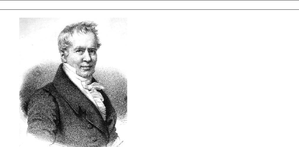
HUMBOLDT, ALEXANDER VON (1759–1859)

Alexander von Humboldt (Figure H13) was born in Berlin in 1769

as the son of a nobleman and former officer of the Prussian Army.

He studied at the universities of Frankfurt/Oder and Göttingen, at the

trade academy of Hamburg and at the mining academy of Freiberg

in Saxonia. In his studies he was interested in all aspects of nature

from botany and zoology to geography and astronomy. His friendship

with Georg Forster who had participated in Cook’s second voyage

and whom he met in Göttingen had a strong influence on him and

402 HUMBOLDT, ALEXANDER VON (1759–1859)

motivated him to see his vocation as a scientific explorer. First he

entered, however, the career as a mining inspector in the service of

the Prussian state. But when his mother died in 1796—he had lost

his father already when he was only nine years old—and he became

the heir of a considerable fortune, he declined the offer of the director-

ship of the Silesian mines and started the realization of his long held

plan for a scientific expedition. In 1798, he embarked on his six years

voyage to South and North America from which he returned in 1804

with huge collections of scientific data and materials. It was in the pre-

paration for this expedition that he was instructed by the French math-

ematician and nautical officer Jean-Charles de Borda in the

measurements of the components of the Earth’s magnetic field and

throughout the years of his voyage he collected magnetic data in addi-

tion to geodetic, meteorological, and other ones. One of his findings

was the decrease of magnetic intensity with latitude which, apparently,

had not been clearly recognized until that time since measurements

had been focused on the direction of the field.

A. von Humboldt continued his magnetic measurements on his voy-

age with his friend Gay-Lussac to Italy in 1805 and back to Berlin.

Here he was offered a wooden cabin, which allowed him to take read-

ings of the declination each night for several months, a task he shared

with the astronomer Oltmann. In December 1805 he was lucky in

observing strong fluctuations of the magnetic field while an aurora

borealis occurred. Humboldt coined the term “Magnetischer Sturm”

for the period of strong oscillations of the magnetometer needle.

Nowadays the term “magnetic storm” is generally accepted for this

phenomenon. Because of the defeat of Prussia by Napoleon’s army

von Humboldt had to stay longer in Berlin than he had planned and

returned to Paris only in late 1807. Here he was occupied with the edi-

tion of the scientific results of his American voyage until 1827. It is

worth noting that during a shorter journey to Berlin in 1826, he

stopped in Göttingen to meet Carl Friedrich Gauss (see Gauss, Carl

Friedrich) for the first time in person.

A. von Humboldt and Gauss were the most prominent German

scientists of their time and they had been in contact by letters for quite

a while. They had high regards for each other even though they were

opposites in their styles of research. A. von Humboldt was one of the

last universally educated scientists interested in the descriptiv e com-

prehension of all natural phenomena, while the mathematician and

physicist Gauss used primarily deductive analysis in his research.

The study of the Earth’s magnetic field was one of their common inter-

ests. Their interaction intensified after von Humboldt had invited

Gauss to participate in the 7th Assembly of the Society of German

Scientists and Physicians, which took place in the fall of 1828 in

Berlin. During that time Gauss stayed at von Humboldt’s house. The

latter had left Paris reluctantly in 1827 to follow a call from the

Prussian King Friedrich Wilhelm III to assume the position of a cham-

berlain at the Berlin court. In his free time, von Humboldt continued

his scientific work among which magnetic measurements had a high

priority. For this purpose his friend A. Mendelson-Bartholdy (father

of the famous composer) had provided a place in his garden where

von Humboldt built an iron free wooden cabin for his magnetometers.

Gauss pursued his studies of the Earth’s magnetic field quite inde-

pendently from those of von Humboldt, which caused the latter some

irritation. Von Humboldt had thought that he had motivated Gauss to

do magnetic measurements when the latter visited him in Berlin in

1828. But Gauss’ interests in geomagnetism went back to a time

40 years earlier, as he mentions in a letter of 1833, and in 1806 he

had already contemplated a description of the field in terms of spheri-

cal harmonics. At the Berlin Assembly, Gauss had met the promising

physicist Wilhelm Weber and had arranged that this young man got

a professorship in Göttingen in 1831. In the following six years, an

intense and highly productive collaboration between Gauss and Weber

ensued on all kinds of electromagnetic problems. In the course of this

research Gauss developed his method of the absolute determination of

magnetic intensity (see Gauss’ determination of absolute intensity) and

built together with Weber appropriate instruments. It now became pos-

sible to calibrate instruments locally independently from any other. For

the purpose of absolute measurements of the magnetic field and its

variations in time at different places on the Earth, Gauss and Weber

initiated the “Göttinger Magnetischer Verein.”

Alexander von Humboldt was also interested in simultaneous mea-

surements of the geomagnetic field at different geographic locations

in order to determine, for instance, whether magnetic storms are of ter-

restrial origin or depended on the position of the Sun. Already in 1828

he had arranged for coincident measurements in Paris and inside a

mine in Freiberg (Saxonia). When he received a glorious reception at

the Russian court at St. Petersburg in 1829 at the end of his expedition

to Siberia, von Humboldt used the opportunity to suggest the creation

of a network of stations throughout the Russian empire for the collec-

tion of magnetic and meteorological data. In the following years such

stations were indeed installed including one in Sitka, Alaska, which at

that time belonged to Russia. Von Humboldt realized that he had to

persuade British authorities in order to achieve his goal of a nearly

worldwide distribution of stations. In 1836 he wrote to the Duke of

Sussex whom he had gotten to know during his student days at the

University of Göttingen and who was now the president of the Royal

Society. For an English translation of this letter see the paper by

Malin and Barraclough (1991). Von Humboldt’s recommendations

for the establishment of permanent magnetic observatories in Canada,

St. Helena, Cape of Good Hope, Ceylon, Jamaica, and Australia were

well received. Besides realizing these proposals, the British Govern-

ment went a step further and organized an expedition to Antarctica

under the direction of Sir James Clark Ross with magnetic measure-

ments as one of its main tasks. Based on the observatory data, Sir

Edward Sabine (see Sabine, Edward) who supervised the network of

stations could later establish a connection between magnetic storms

and sunspots and demonstrate in particular the correlation between

the 11-year sunspot cycle and a corresponding periodicity of magnetic

storms.

In the course of his continuing research on geomagnetism, von

Humboldt realized the superiority of Gauss’ method of measurement

and he also often expressed his admiration for Gauss

’ theoretical work

on the representation of the geomagnetic field in terms of potentials

and the separation of internal and external sources in particular. From

today’s point of view it is obvious that Gauss made the more funda-

mental contributions to the field of geomagnetism. But Alexander

Figure H13 Alexander von Humboldt in 1832. (Lithography of

F.S. Delpech after a drawing of Francois Ge

rard.)

HUMBOLDT, ALEXANDER VON (1759–1859) 403

von Humboldt ’s lasting legacy has been the organization of a world-

wide cooperation in the gathering of geophysical data with simulta-

neous measurements at prearranged dates; the influence of which can

still be felt today. A. von Humboldt died in 1859 at the age of nearly

90 years. For further details on von Humboldt’s scientific endeavours

the reader is referred to the book by Botting (1973).

Friedrich Busse

Bibliography

Botting, D., 1973. Humboldt and the Cosmos, George Rainbird Ltd.,

London.

Malin, S.R.C. and Barraclough, D.R., 1991. Humboldt and the Earth’s

magnetic field Quarterly Journal of the Royal Astronomical

Society 32: 279–293.

Cross-references

Gauss, Carl Friedrich (1777–1855)

Gauss’ Determination of Absolute Intensity

Sabine, Edward (1788–1883)

HUMBOLDT, ALEXANDER VON AND

MAGNETIC STORMS

Baron Alexander von Humboldt (September 14, 1769–May 6, 1859)

was a great German naturalist and explorer, universal genius and cos-

mopolitan, scientist, and patron. Application of his experience and

knowledge gained through his travels and experiments transformed

contemporary western science. He is widely acknowledged as the

founder of modern geography, climatology, ecology, and oceanogra-

phy. This article focuses on Alexander von Humboldt’s contribution

to the science of geomagnetism (Busse, 2004), which is not so widely

known.

Historical background on geomagnetism

With the publication of De Magnete by William Gilbert in A.D. 1600,

the Earth itself was seen as a great magnet, and a new branch of phy-

sics, geomagnetism, was born. The first map of magnetic field declina-

tion was made by Edmund Halley in the beginning of 18th century.

Alexander von Humboldt prepared a chart of “isodynamic zones” in

1804, based on his measurements made during his voyages through

the Americas (1799–1805). He swung a dip needle in the magnetic

meridian plane, and observed the number of oscillations during

10 min. He noticed that the number of oscillations were at maximum

near the magnetic equator, and decreased to the north and to the south.

This indicated a regular decrease of the total magnetic intensity from

the poles to the equator. The publication of this result stimulated

further investigations on the Earth’s magnetic field (Chapman and

Bartels, 1940). Von Humboldt, together with Guy Lussac, improvised

the method to measure the horizontal intensity by observing the time

of oscillation of a compass needle in the horizontal plane. They took

the first measurements of the relative horizontal intensity of the Earth’s

magnetic field on a journey to Italy in 1807.

From May 1806 to June 1807 in Berlin, Humboldt and a colleague

observed the local magnetic declination every half hour from midnight

to morning. On December 21, 1806, for six consecutive hours, von

Humboldt observed strong magnetic deflections and noted the presence

of correlated northern lights (aurora) overhead. When the aurora disap-

peared at dawn, the magnetic perturbations disappeared as well. Von

Humboldt concluded that the magnetic disturbances on the ground

and the auroras in the polar sky were two manifestation of the same

phenomenon (Schröder, 1997). He gave this phenomenon involving

large-scale magnetic disturbances (possibly already observed by

George Graham) the name “Magnetische Ungewitter,” or magnetic

storms (von Humboldt, 1808). The worldwide net of magnetic observa-

tories later confirmed that such “storms” were indeed worldwide

phenomena.

Alexander von Humboldt organized the first simultaneous observa-

tions of the geomagnetic field at various locations throughout the

world after his return from his South American journey. Wilhelm

Weber, Karl F. Gauss, and he organized the Göttingen Magnetische

Verein (Magnetic Union); and from 1836–1841, simultaneous obser-

vations of the Earth’s magnetic field were made in nonmagnetic huts

at up to 50 different locations, marking the beginning of the magnetic

observatory system. Through his diplomatic contacts, Alexander von

Humboldt was instrumental in the establishment of a number of mag-

netic observatories around the world, especially in Britain, Russia, and

in countries then under the British and Russian rule, e.g., cities such as

Toronto, Sitka, and Bombay, etc. He constructed his own iron-free

magnetic observatory in Berlin in 1832. These observatories have

played an important role in the development of the science of geomag-

netism. With the beginning of the space age, our knowledge about the

near-Earth space environment, the magnetosphere-ionosphere sys-

tem in general, and geomagnetic storms in particular, has improved

dramatically.

Intense geomag netic storms and their causes

A geomagnetic storm is characterized by a main phase during which

the horizontal component of the Earth ’s low-latitude magnetic fields

are significantly depressed over a time span of one to a few hours. This

is followed by a recovery phase, which may extend for 10 h or more

(Rostoker, 1997). The intensity of a geomagnetic storm is measured in

terms of the disturbance storm-time index (Dst). Magnetic storms with

Dst < 100 nT are called intense and those with Dst < 500 nT are

called superintense. Geomagnetic storms occur when solar wind-mag-

netosphere coupling becomes intensified during the arrival of fast

moving solar ejecta like interplanetary coronal mass ejections (ICMEs)

and fast streams from the coronal holes (Gonzalez et al., 1994) accom-

panied by long intervals of southward interplanetary magnetic field

(IMF) as in a “magnetic cloud” (Klein and Burlaga, 1982). It is now

well established that the major mechanism of energy transfer from

the solar wind to the Earth’s magnetosphere is magnetic reconnection

(Dungey, 1961). The efficiency of the reconnection process is con-

siderably enhanced during southward IMF intervals (Tsurutani and

Gonzalez, 1997), leading to strong plasma injection from the magneto-

tail towards the inner magnetosphere causing intense auroras at high-

latitude nightside regions. Further, as the magnetotail plasma gets

injected into the nightside magnetosphere, the energetic protons drift

to the west and electrons to the east, forming a ring of current around

the Earth. This current, called the “ring current,” causes a diamagnetic

decrease in the Earth’s magnetic field measured at near-equatorial

magnetic stations (see Figure H14 for the results from one such sta-

tion). The decrease in the equatorial magnetic field strength, measured

by the Dst index, is directly related to the total kinetic energy of

the ring current particles (Dessler and Parker, 1959; Sckopke, 1966);

thus the Dst index is a good measure of the energetics of the mag-

netic storm. The Dst index itself is influenced by the interplanetary

parameters (Burton et al., 1975).

One obviously cannot directly determine the solar/interplanetary

causes of storm events prior to the space age. However, based on the

recently gained knowledge on solar, interplanetary, and magneto-

spheric physics, one can make these determinations by a process of

elimination. For example, by examining the profile of magnetic storms

using ground magnetic field data, storm generation mechanisms can

be identified (Tsurutani et al., 1999). From the ground magnetometer

data shown in Figure H14, reports on the related solar flare event

(Carrington, 1859; Hodgson, 1859), and reports on the concomitant

aurora (taken from newspapers and private correspondence, Kimball,

404 HUMBOLDT, ALEXANDER VON AND MAGNETIC STORMS

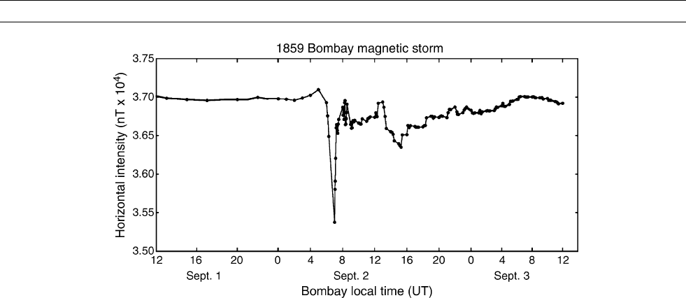
1960), Tsurutani et al. (2003) were able to deduce that an exception-

ally fast (and intense) magnetic cloud was the interplanetary cause of

the superintense geomagnetic storm of September 1–2, 1859 with a

Dst –1760 nT. This large value of Dst is consistent with the decrease

of DH ¼ 1600  10 nT recorded at Colaba (Bombay), India (Figure

H14). The supposition that the intense southward IMF was due to a

magnetic cloud was surmised by the simplicity and short duration of

the storm in the ground magnetic field data. Main phase compound

events or “double storms” (Kamide et al., 1998) can be ruled out by

the (simple) storm profile. Compound stream events (Burlaga et al.,

1987) can also be eliminated by the storm profile. The only other pos-

sibility that might be the cause of the storm is sheath fields associated

with an ICME. This can be ruled out because the compression factor

of magnetic fields following fast shocks is only approximately four

times (Kennel et al., 1985). Thus with quiet interplanetary fields being

typically 3 to 10 nT, the compressed fields would be too low to gen-

erate the inferred interplanetary and magnetospheric electric fields for

the storm. Thus by a process of elimination the interplanetary fields that

caused this superintense storm have been determined to be part of a

fast, intense magnetic cloud.

Geomagnetic storms produce severe disturbances in Earth’s magne-

tosphere and ionosphere, creating so-called adverse space weather

conditions. They pose major threats to space- and ground-based tech-

nological systems on which modern society is becoming increasingly

dependent. The intense magnetic storms during October 29–31,

2003, the so-called “Halloween storms”, associated with the largest

X-ray solar flare of the solar cycle 23, caused damage to 28 satellites,

ending the operational life of two, disturbed flight routes of some air-

lines, telecommunications problems, and power outage in Sweden.

These Halloween storms with Dst –400 nT were about four times

less intense than the superintense storm of 1859. One can imagine

the loss to society if a magnetic storm similar to the superintense storm

of 1859 were to occur today!

Acknowledgments

GSL would like to thank Prof. Y. Kamide for the kind hospitality during

his stay at STEL, Nagoya University, Japan. Portions of the research for

this work were performed at the Jet Propulsion Laboratory, California

Institute of Technology, under contract with the National Aeronautics

and Space Administration.

G.S. Lakhina, B.T. Tsurutani, W.D. Gonzalez, and S. Alex

Bibliography

Burlaga, L.F., Behannon, K.W., and Klein, L.W. 1987. Compound

streams, magnetic clouds, and major geomagnetic storms. Journal

of Geophysical Research, 92: 5725.

Burton, R.K., McPherron, R.L., and Russell, C.T. 1975. An empirical

relationship between interplanetary conditions and Dst. Journal of

Geophysical Research, 80: 4204.

Busse, F., 2004. Alexander von Humboldt, this volume.

Carrington, R.C., 1859. Description of a singular appearance seen in

the Sun on September 1, 1859. Monthly Notices of the Royal Astro-

nomical Society, XX, 13.

Chapman, S. and Bartels, J., 1940. Geomagnetism, vol. II, Oxford

University Press, New York, pp. 913–933.

Dessler, A.J., and Parker, E.N., 1959. Hydromagnetic theory of mag-

netic storms. Journal of Geophysical Research, 64: 2239.

Dungey, J.W., 1961. Interplanetary magnetic field and the auroral

zones. Physical Research Letters, 6 : 47.

Gonzalez, W.D., Joselyn, J.A., Kamide, Y., Kroehl, H.W., Rostoker, G.,

Tsurutani, B.T., and Vasyliunas, V.M., 1994. What is a geomagnetic

storm? Journal of Geophysical Research, 99: 5771.

Hodgson, R.,1859. On a curious appearance seen in the Sun. Monthly

Notices of the Royal Astronomical Society London, XX, 15.

Kamide, Y., Yokoyama, N., Gonzalez, W., Tsurutani, B.T., Daglis, I.A.,

Brekke, A., and Masuda, S., 1998. Two-step development of geo-

magnetic storms. Journal of Geophysical Research, 103: 6917.

Kennel, C.F., Edmiston, J.P., and Hada, T. 1985. A quarter century of

collisionless shock research. In Stone, R.G. and Tsurutani, B.T.

(eds.), Collisionless Shocks in the Heliosphere: A Tutorial Review.

Washington, DC: American. Geophysical Union, Vol. 34, p. 1.

Kimball, D.S., 1960. A study of the aurora of 1859. Sci. Rpt. 6, UAG-

R109, University of Alaska.

Klein, L.W. and Burlaga, L.F., 1982. Magnetic clouds at 1 AU. Jour-

nal of Geophysical Research, 87: 613.

Rostoker, G., 1997. Physics of magnetic storms. In Tsurutani, B.T.,

Gonzalez, W.D., Kamide, Y., and Arballo, J.K. (eds.), Magnetic

Storms. Geophysical Monograph 98, AGU, Washington DC, p. 149.

Schröder, W., 1997. Some aspectss of the earlier history of solar-

terrestrial physics. Planetary and Space Science, 45: 395.

Sckopke, N., 1966. A general relation between the energy of trapped

particles and the disturbance field near the Earth. Journal of

Geophysical Research, 71: 3125.

Tsurutani, B.T. and Gonzalez, W.D., 1997. Interplanetary causes of

magnetic storms: a review. In Tsurutani, B.T., Gonzalez, W.D.,

Figure H14 The Colaba (Bombay) magnetogram for the September 1–2, 1859 geomagnetic storm. The peak near 0400 UT September

2, is due to the storm sudden commencement (SSC) caused probably by the shock ahead of the magnetic cloud. This was followed

by the storm “main phase” which lasted for about one hour and a half. Taken from Tsurutani et al. (2003).

HUMBOLDT, ALEXANDER VON AND MAGNETIC STORMS 405