Gubbins D., Herrero-Bervera E. Encyclopedia of Geomagnetism and Paleomagnetism

Подождите немного. Документ загружается.

In the case that Y ¼ 0, and the spherical triangle collapses to a straight

line so that b ¼ y and f ¼ a , then since P

ð 1Þ¼1 for all values of l,

then Eq. (98) becomes

M ¼l

ð y ; f Þ Y

ðy ; f Þ¼2 l þ 1 : (Eq. 103)

and Eq. (100) in terms of Schmidt normalized polynomials gives

M ¼ 0

ðcos yÞ



¼ 1 ; (Eq. 104)

which can be used to provide a useful check on numerical work.

The result of Eq. (103) is equivalent to the conservation of “lengths ”

under rotation, and therefore requires that the ð 2 l þ 1 Þð2l þ 1 Þ rota-

tion matrices D

ð a ; b; gÞ be unitary, i.e.,

M ¼l

ða ; b ; g Þ D

ð a; b; gÞ¼ d

: (Eq. 105)

Schmi dt’s analysis

Schmidt (1899) derived the transformation formula (83) for spherical

harmonics well before the later derivations in the context of the theory

of atomic spectra. Schmidt gave the result in terms Schmidt normal-

ized functions, using real variables only, as

ðcos Y Þ cos m½p ðF þ gÞ

M ¼ 0

ﬃﬃﬃﬃﬃﬃﬃﬃﬃﬃ

ð 1Þ

M ;m

ð bÞþ d

 M ;m

ð bÞ

 P

ðcos yÞ cos M ðf  a Þ: (Eq: 106)

Because m and M ¼ 1 ; 2 ; 3 ;... only in the expression for imaginary

component, therefo re, in this case, e

¼ 2 and e

¼ 2, and

ð cos Y Þ sin m½p ðF þ gÞ

M ¼1

ð 1 Þ

M ;m

ð bÞd

M ; m

ðb Þ

ð cos y Þ sin M ð f  a Þ

(Eq. 107)

The expression Schmidt developed for the rotation matrix elements

was given in a slightly different, but nevertheless equivalent form to

that of Eq. (89) where z ¼ cos b. In Schmidt ’s result, c ¼ cos b and

s ¼ sin b , and

ð bÞ¼ð1 Þ

ﬃﬃﬃﬃﬃﬃﬃﬃﬃﬃﬃﬃﬃﬃﬃﬃﬃﬃﬃﬃﬃﬃﬃﬃﬃﬃﬃﬃﬃﬃﬃﬃﬃ

ð l  m Þ!ðl  M Þ!

ð l þ m Þ!ðl þ M Þ!

ð1 þ c Þ

M m

d c



ð1  c Þ

d c



ðc Þ



: (Eq. 108)

Leibnitz ’s theorem is used to show the equivalence of Eqs. (108) and

(89), where z ¼ cos b .

Wigne r 3- j coeffic ients

The Wigner 3- j coefficients (Wigner, 1931) are just generalizations of

the factors that appear in recurrence relations for associated Legendre

polynomials, and rotation matrix elements. They have an interesting

structure, and are best defined as a sum of products of three combina-

torial coefficients. Thus

abc

abg



¼ð1 Þ

ab g

ﬃﬃﬃﬃﬃﬃﬃﬃﬃﬃﬃﬃﬃﬃﬃﬃﬃﬃﬃﬃﬃﬃﬃﬃﬃﬃﬃﬃﬃﬃﬃﬃﬃﬃﬃﬃﬃﬃﬃﬃﬃﬃﬃﬃﬃﬃﬃﬃﬃﬃﬃﬃﬃﬃﬃﬃﬃﬃﬃﬃﬃﬃﬃﬃﬃﬃﬃﬃﬃﬃﬃﬃﬃﬃﬃﬃﬃﬃﬃﬃﬃﬃﬃﬃﬃﬃﬃﬃﬃﬃﬃﬃﬃﬃ

ð a  aÞ!ð a þ aÞ!ð b  bÞ!ð b þ b Þ!ð c  g Þ!ð c þ g Þ!

ð a þ b þ c Þ!ð a  b þ c Þ!ð a þ b  c Þ!



ﬃﬃﬃﬃﬃﬃﬃﬃﬃﬃﬃﬃﬃﬃﬃﬃﬃﬃﬃﬃﬃﬃﬃﬃﬃﬃﬃﬃﬃﬃﬃﬃ

ð a þ b þ c þ 1Þ!

ð1Þ

a  b þ c

a  a  t



a þ b þ c

b þ b  t



a þ b  c



(Eq. 109)

Conditi ons on the values of the parameters require that the nine

elements of the following 3  3 array, called a Racah square, are all

positive,

 a þ b þ ca b þ caþ b  c

a  a b  b c  g

a þ a b þ b c þ g

(Eq. 110)

and that a þ b þ g ¼ 0. The following special cases of the 3- j

coefficients are determined from the series definition of Eq. (109),

llþ 11

m m  11



¼ð1Þ

l m

ﬃﬃﬃﬃﬃﬃﬃﬃﬃﬃﬃﬃﬃﬃﬃﬃﬃﬃﬃﬃﬃﬃﬃﬃﬃﬃﬃﬃﬃﬃﬃﬃﬃﬃﬃﬃﬃﬃﬃﬃﬃﬃﬃﬃﬃﬃﬃﬃ

ð l þ m þ 1 Þðl þ m þ 2 Þ

ð2 l þ 1 Þð2 l þ 2Þð 2l þ 3 Þ

;

llþ 11

m m 0



¼ð1 Þ

l  m 1

ﬃﬃﬃﬃﬃﬃﬃﬃﬃﬃﬃﬃﬃﬃﬃﬃﬃﬃﬃﬃﬃﬃﬃﬃﬃﬃﬃﬃﬃﬃﬃﬃﬃﬃﬃﬃﬃﬃﬃﬃﬃﬃﬃﬃﬃﬃﬃﬃ

2 ðl  m þ 1 Þðl þ m þ 1 Þ

ð 2l þ 1 Þð2l þ 2 Þð2 l þ 3 Þ

;

llþ 11

m m þ 1  1



¼ð1 Þ

l m

ﬃﬃﬃﬃﬃﬃﬃﬃﬃﬃﬃﬃﬃﬃﬃﬃﬃﬃﬃﬃﬃﬃﬃﬃﬃﬃﬃﬃﬃﬃﬃﬃﬃﬃﬃﬃﬃﬃﬃﬃﬃﬃﬃﬃﬃﬃﬃﬃ

ð l  m þ 1 Þðl  m þ 2Þ

ð2 l þ 1Þð2 l þ 2 Þð2l þ 3 Þ

;

(Eq. 111)

ll1

m m  11



¼ð1Þ

l m

ﬃﬃﬃﬃﬃﬃﬃﬃﬃﬃﬃﬃﬃﬃﬃﬃﬃﬃﬃﬃﬃﬃﬃﬃﬃﬃﬃﬃﬃﬃﬃﬃﬃﬃﬃﬃﬃﬃﬃﬃ

2ð l  m Þðl þ m þ 1Þ

2ð 2 l þ 1 Þð2 l þ 2 Þ

;

ll1

m m 0



¼ð1Þ

l  m

ﬃﬃﬃﬃﬃﬃﬃﬃﬃﬃﬃﬃﬃﬃﬃﬃﬃﬃﬃﬃﬃﬃﬃﬃﬃﬃﬃﬃﬃﬃﬃﬃﬃﬃﬃﬃ

2 l ð 2l þ 1 Þð2 l þ 2 Þ

;

ll 1

m m þ 1  1



¼ð1 Þ

l þm 1

ﬃﬃﬃﬃﬃﬃﬃﬃﬃﬃﬃﬃﬃﬃﬃﬃﬃﬃﬃﬃﬃﬃﬃﬃﬃﬃﬃﬃﬃﬃﬃﬃﬃﬃﬃﬃﬃﬃﬃﬃ

2ð l þ mÞðl  m þ 1Þ

2l ð 2 l þ 1 Þðl þ 2Þ

;

(Eq. 112)

ll 11

m m  11



¼ð1 Þ

l  m

ﬃﬃﬃﬃﬃﬃﬃﬃﬃﬃﬃﬃﬃﬃﬃﬃﬃﬃﬃﬃﬃﬃﬃﬃﬃﬃﬃﬃﬃﬃﬃﬃﬃﬃﬃﬃﬃﬃ

ð l  m  1 Þðl  mÞ

ð 2l  1 Þ2 l ð 2l þ 1 Þ

;

ll 11

m m 0



¼ð1Þ

l m

ﬃﬃﬃﬃﬃﬃﬃﬃﬃﬃﬃﬃﬃﬃﬃﬃﬃﬃﬃﬃﬃﬃﬃﬃﬃﬃﬃﬃﬃﬃﬃﬃﬃﬃﬃﬃ

2 ðl  mÞð l þ m Þ

ð2 l  1 Þ 2l ð 2 l þ 1 Þ

;

ll 11

m m þ 1 1



¼ð1 Þ

l  m

ﬃﬃﬃﬃﬃﬃﬃﬃﬃﬃﬃﬃﬃﬃﬃﬃﬃﬃﬃﬃﬃﬃﬃﬃﬃﬃﬃﬃﬃﬃﬃﬃﬃﬃﬃﬃﬃﬃ

ð l þ m  1 Þðl þ mÞ

ð 2 l  1 Þ 2l ð 2 l þ 1 Þ

;

(Eq. 113)

An integration formula

The following integration formula can be used to derive the properties

of 3-j coefficients directly from their definitions,

1

ðm  1Þ

m

ðm þ 1Þ

þm



þl

l

ðm  1Þ

m

ðm þ 1Þ

þm

¼ð1Þ

ðl

þ l

 l

Þ!





ðl

 m

Þ!ðl

þ m

Þ!ðl

 m

Þ!ðl

þ m

Þ!ðl

 m

Þ!ðl

þ m

Þ!

ðl

þ l

 l

Þ!ðl

 l

þ l

Þ!ðl

þ l

Þ!ðl

þ l

Þ!



(Eq. 114)

386 HARMONICS, SPHERICAL

The 3- j coefficients have two important orthogonality properties

þm

þ m

¼ 0



þ 1

;

(Eq. 115)

and Eq. (119) given below.

Produ cts of ro tation matrix elements

The integral of a product of three rotation matrix elements is

8 p

2 p

sin bd ad b dg



(Eq: 116)

and therefore, from the orthogonality of rotation matrix elements, it

follows that the product of two rotation matrix elements can be written

as a sum of rotation matrix elements,

ða ; b ; gÞD

ða ; b ; gÞ

ð2 l

þ 1 Þ



ða ; b ; gÞ:

(Eq. 117)

Equation (117) is an important equation because it effectively contains

all the recurrence relations for rotation matrix elements, and therefore

for surface spherical harmonics. The first orthogonality property of 3- j

coefficients applied to the product formula (117) gives



(Eq. 118)

Setting a ¼ b ¼ g ¼ 0 in Eq. (117) gives the second orthogonality

property of the 3- j coefficients,

ð2 l

þ 1 Þ



¼ d

(Eq. 119)

Vector cou pling coeffic ients

In applications, it is more convenient to use a coupling coefficient,

(Varshalovich et al., 1988),

;m

¼ð1 Þ

l

m

ﬃﬃﬃﬃﬃﬃﬃﬃﬃﬃﬃﬃﬃﬃ

2 l

þ 1



; (Eq. 120)

when the orthogonality properties, Eqs. (115) and (119) are

þm

¼ m

¼ d

; with m

þ m

¼ m

;

(Eq. 121)

¼ d

; with m

þ m

¼ m

; m

þ m

¼ m

(Eq. 122)

The product formulae (117) and (118), for rotation matrix elements

become

; m

; (Eq. 123)

¼ C

; (Eq. 124)

respectively, and in both of which

þ M

¼ M

; and m

þ m

¼ m

Note that the complex conjugate expressions required on the right-hand

sides of Eqs. (117) and (118) are not required in the corresponding vector

couplin g coefficient formulae. This occurs because of the result that

 M ; m

ð a ; b ; gÞ¼ð1Þ

M  m

M ;m

ð a; b; g Þ: (Eq. 125)

We can now use vector-coupling coefficient to couple together two

quantities that transform like spheri cal harmonics. Consider

ðY

; F

Þ¼

¼l

; m

ða ; b ; g ÞY

ð y

; f

Þ;

ðY

; F

Þ¼

¼l

; m

ða ; b ; g ÞY

ð y

; f

Þ: (Eq: 126)

When the coupled spherical harmonic expression is formed

ðY

; F

ÞY

ðY

; F

¼ l

¼l

 Y

ð y

; f

ÞY

ð y

; f

Þ: (Eq: 127)

The sums on the right of Eq. (127) can be rearranged and the expres-

sions in square brackets replaced by means of Eq. (124), givin g the

results that

ð Y

; F

Þ Y

ð Y

; F

ðy

; f

Þ Y

ðy

; f

;

(Eq: 128)

showing that the coupled expression in square brackets in Eq. (128)

obeys the transformation law for spherical harmonics Y

ð Y ; F Þunder

rotation of the reference frame; that is

ð Y ; FÞ¼

ð y

; f

ÞY

ð y

; f

Þ; (Eq. 129)

so that coupled spherical harmonics on the right of Eq. (129) will trans-

form under rotation of the reference frame like a spherical harmonics.

Vector spherical harmonics

If the unit vectors in the x-, y- and z-directions are denoted e

; e

;

respectively, the complex reference vectors e

; e

1

; are defined by

HARMONICS, SPHERICAL 387

¼

ﬃﬃﬃ

ð e

þ i e

Þ¼rx ;

¼ e

¼rz ;

1

ﬃﬃﬃ

ð e

 i e

Þ¼r: (Eq: 130)



denotes the complex conjugate of e

; m ¼1 ; 0 ; 1 ; then the

complex reference vectors satisfy



¼ d

; and e

 e

¼ð1Þ

m n

n

; for m ; n ¼ 1 ; 0 ;1 :

(Eq. 131)

Therefore, a vector B, with Cartesian components B

; B

; will have

complex reference components B

1

; B

; such that B ¼B

1

 B

1

; and

¼

ﬃﬃﬃ

ð B

þ iB

Þ;

¼ B

;

1

ﬃﬃﬃ

ð B

 iB

Þ: (Eq: 132)

Complex reference components of the gradient operator r and the

angular momentum operator L ¼i r r, are obtained, and can be

expressed in terms of spherical polar coordinates, r ; y ; f ; as follows:

¼

ﬃﬃﬃ

sin y

]

] r

cos y

]

] y

r sin y

]

] f



;

¼ cos y

]

] r



sin y

]

;

 1

ﬃﬃﬃ

 if

sin y

]

cos y

]

] y



r sin y

]

] f



; (Eq: 133)

and

¼

ﬃﬃﬃ

]

] y

þ i cot y

]

] f



;

¼i

]

] f

;

1

¼

ﬃﬃﬃ

i f

]

] y

 i cot y

]

] f



: (Eq: 134)

We now define three vector spherical harmonics

l ;l þ1

ðy ; f Þ; Y

l ;l

ð y ; f Þ; Y

l ; l  1

ð y; fÞ; in terms of complex reference vec-

tors, and also present them in the better known and widely used forms

in terms of spherical polars. Thus

l þ 2

ﬃﬃﬃﬃﬃﬃﬃﬃﬃﬃﬃﬃﬃﬃﬃﬃﬃﬃﬃﬃﬃﬃﬃﬃﬃﬃﬃﬃﬃﬃ

ð l þ 1Þð2 l þ 1 Þ

l ;l þ 1

ðy ; f Þ¼r

l þ 1

ð y; fÞ



;

ﬃﬃﬃﬃﬃﬃﬃﬃﬃﬃﬃﬃﬃﬃﬃ

l ð l þ 1Þ

l ;l

ðy ; f Þ¼ LY

ð y; fÞ;

l 1

ﬃﬃﬃﬃﬃﬃﬃﬃﬃﬃﬃﬃﬃﬃﬃﬃﬃﬃ

l ð2 l þ 1 Þ

l ;l  1

ðy ; f Þ¼r r

ð y; fÞ



(Eq. 135)

The spherical polar components of the vector spherical harmonics are

ﬃﬃﬃﬃﬃﬃﬃﬃﬃﬃﬃﬃﬃﬃﬃﬃﬃﬃﬃﬃﬃﬃﬃﬃﬃﬃﬃﬃﬃ

ðl þ1Þð2l þ1Þ

l;lþ1

ðy; fÞ¼ðl þ1ÞY

sin y

;

ﬃﬃﬃﬃﬃﬃﬃﬃﬃﬃﬃﬃﬃﬃﬃ

lðl þ1Þ

l;l

ðy; fÞ¼

sin y

i

;

ﬃﬃﬃﬃﬃﬃﬃﬃﬃﬃﬃﬃﬃﬃﬃﬃﬃ

lð2l þ1Þ

l;l1

ðy; fÞ¼lY

siny

;

(Eq. 136)

where e

; e

; are unit vectors in the direction of r; y; f; increasing,

respectively.

However, from the recurrence relations given in Eqs. (64) – (71),

and from the spherical polar forms of the vector operators given in

Eqs. (133) and (134), it follows immediately that

ﬃﬃﬃﬃﬃﬃﬃﬃﬃﬃﬃﬃﬃﬃﬃﬃﬃﬃﬃﬃﬃﬃﬃﬃﬃﬃﬃﬃﬃﬃ

ðl þ 1Þð2l þ 1Þ

l;lþ1

ﬃﬃﬃﬃﬃﬃﬃﬃﬃﬃﬃﬃﬃ

2l þ 1

2l þ 3



ﬃﬃﬃ

ﬃﬃﬃﬃﬃﬃﬃﬃﬃﬃﬃﬃﬃﬃﬃﬃﬃﬃﬃﬃﬃﬃﬃﬃﬃﬃﬃﬃﬃﬃﬃﬃﬃﬃﬃﬃﬃﬃﬃﬃﬃﬃﬃﬃﬃﬃ

ðl þ m þ 1Þðl þ m þ 2Þ

mþ1

lþ1



1



ﬃﬃﬃﬃﬃﬃﬃﬃﬃﬃﬃﬃﬃﬃﬃﬃﬃﬃﬃﬃﬃﬃﬃﬃﬃﬃﬃﬃﬃﬃﬃﬃﬃﬃﬃﬃﬃﬃﬃﬃﬃﬃﬃﬃﬃﬃ

ðl  m þ 1Þðl þ m þ 1Þ

lþ1

ﬃﬃﬃ

ﬃﬃﬃﬃﬃﬃﬃﬃﬃﬃﬃﬃﬃﬃﬃﬃﬃﬃﬃﬃﬃﬃﬃﬃﬃﬃﬃﬃﬃﬃﬃﬃﬃﬃﬃﬃﬃﬃﬃﬃﬃﬃﬃﬃﬃﬃ

ðl  m þ 1Þðl  m þ 2Þ

lþ1



;

(Eq. 137)

ﬃﬃﬃﬃﬃﬃﬃﬃﬃﬃﬃﬃﬃﬃﬃ

lðl þ 1Þ

l;l

ﬃﬃﬃ

ﬃﬃﬃﬃﬃﬃﬃﬃﬃﬃﬃﬃﬃﬃﬃﬃﬃﬃﬃﬃﬃﬃﬃﬃﬃﬃﬃﬃﬃﬃﬃﬃﬃﬃﬃﬃﬃﬃ

ðl þ m þ 1Þðl  mÞ

mþ1

1

þ mY



ﬃﬃﬃ

ﬃﬃﬃﬃﬃﬃﬃﬃﬃﬃﬃﬃﬃﬃﬃﬃﬃﬃﬃﬃﬃﬃﬃﬃﬃﬃﬃﬃﬃﬃﬃﬃﬃﬃﬃﬃﬃﬃ

ðl þ mÞðl  m þ 1Þ

m1

;

(Eq. 138)

ﬃﬃﬃﬃﬃﬃﬃﬃﬃﬃﬃﬃﬃﬃﬃﬃﬃﬃ

lð2l þ 1Þ

l;l1

ﬃﬃﬃﬃﬃﬃﬃﬃﬃﬃﬃﬃﬃ

2l þ 1

2l  1

ﬃﬃﬃ



ﬃﬃﬃﬃﬃﬃﬃﬃﬃﬃﬃﬃﬃﬃﬃﬃﬃﬃﬃﬃﬃﬃﬃﬃﬃﬃﬃﬃﬃﬃﬃﬃﬃﬃﬃﬃﬃﬃ

ðl  m  1Þðl  mÞ

mþ1

l1

1

ﬃﬃﬃﬃﬃﬃﬃﬃﬃﬃﬃﬃﬃﬃﬃﬃﬃﬃﬃﬃﬃﬃﬃﬃﬃﬃﬃﬃﬃ

ðl þ mÞðl  mÞ

l1

ﬃﬃﬃ

ﬃﬃﬃﬃﬃﬃﬃﬃﬃﬃﬃﬃﬃﬃﬃﬃﬃﬃﬃﬃﬃﬃﬃﬃﬃﬃﬃﬃﬃﬃﬃﬃﬃﬃﬃﬃﬃﬃ

ðl þ m  1Þðl þ mÞ

m1

l1



(Eq. 139)

Using the 3- j coefficients listed in Eqs. (111) –(113), it follows that all

three Eqs. (137) –(139) can be written as a single expression

l;lþn

ðy; fÞ¼ð1Þ

lþn1þm

ﬃﬃﬃﬃﬃﬃﬃﬃﬃﬃﬃﬃﬃ

2l þ 1

m¼1

l þ n 1 l

m  mmm



mm

lþn

(Eq. 140)

In terms of the coupling coefficient of Eq. (120)

l;lþn

ðy; fÞ¼

m¼1

l;m

lþn;mm;1;m

mm

lþn

: (Eq. 141)

Because of the orthogonality properties of complex reference vectors

and surface spherical harmonics, it follows that the vector spherical har-

monics are orthogonal under integration over the surface of a sphere:

þm

ðy; fÞY

þn

ðy; fÞsin ydydf ¼ d

(Eq. 142)

Appendix

Rotations

Introduction

The word “rotation” has related, but nevertheless, different meanings

in different disciplines, such as agriculture, medicine, psychology,

and mechanics. This article is intended to deal with the theory of rota-

tion about an axis, and to bring together the relationships between the

388 HARMONICS, SPHERICAL

different methods used to describe rotations, including the angle

and axis of rotation, the Euler-Rodrigues parameters, quaternions, the

Cayley-Klein parameters, spinors, and Euler angles.

Rotation ab out an axis

Consider a positive rotation of a system of particles without deforma-

tion, through an angle V about an axis n, in a reference frame that

remains fixed. An origin O is chosen along the axis of rotation, and

r is the positio n vector of a general particle that becomes the vector

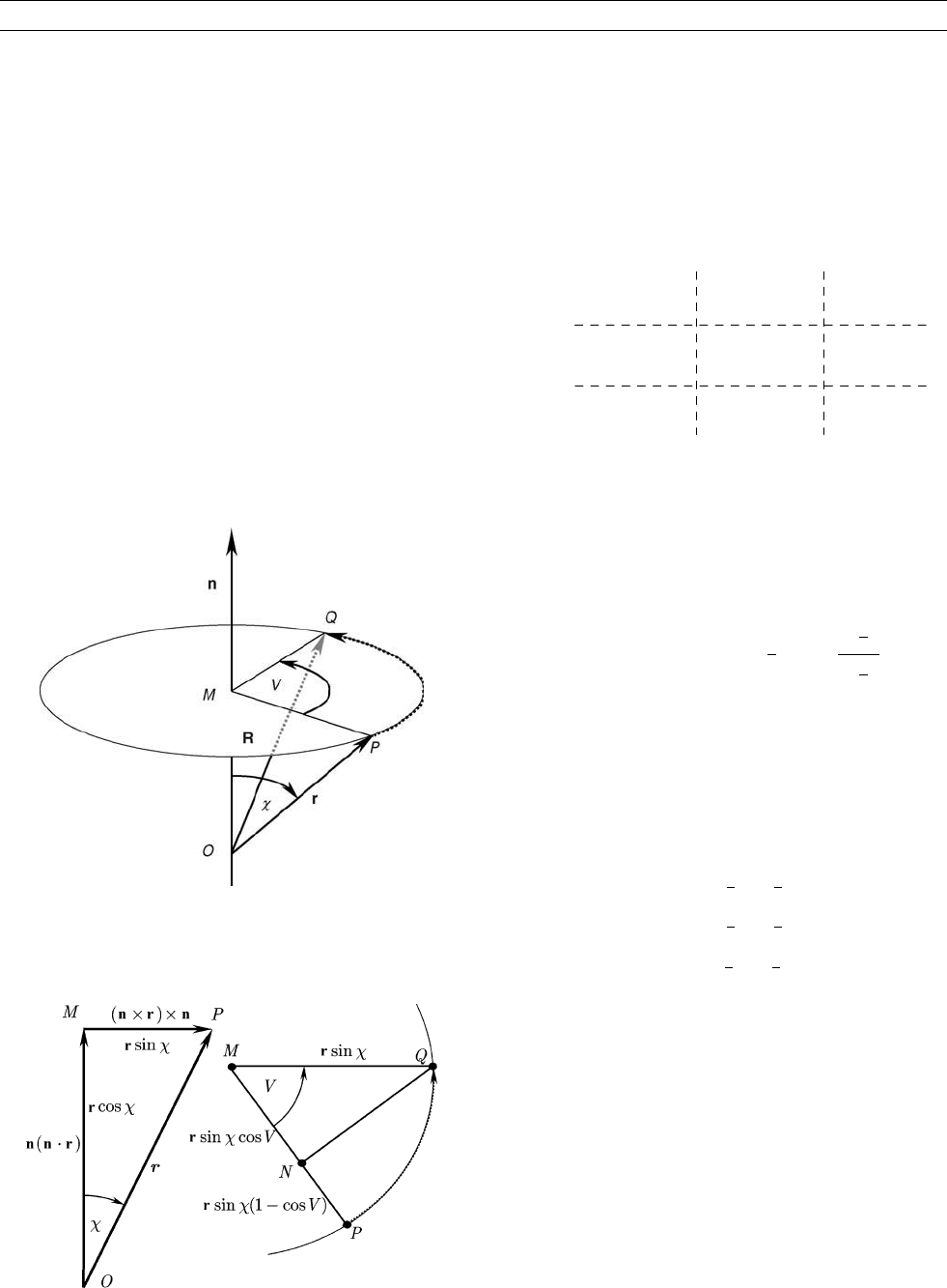
R. From Figures H5 and H6, it can be seen that

R ¼ OQ

!

¼ OP

!

þ PN

!

þ NQ

!

;

¼ r þðn  rÞn½ðcos V  1Þþðn  r Þ sin V : (Eq: 143)

where N is a point along PM, such that PN is perpendicular to NQ.

Therefore,

R ¼ r cos V þ n ðn  r Þð1  cos V Þþðn  r Þ sin V : (Eq. 144)

Rotation of the reference frame

The equation for the transformation of the coordinates of P, under rota-

tion of the reference frame, follows directly from Eq. (144) by chan-

ging the sign of the angle V. Thus

R ¼ r cos V þnðn  rÞð1  cos VÞðn  rÞsin V : (Eq. 145)

Writing out the Cartesian components of Eq. (145) gives a matrix form

R ¼ A  r; where A ¼ Aðn; V Þ; and (Eq. 146)

Aðn; V Þ¼

cos Vabð1  cos V Þ acð1  cos V Þ

þa

ð1  cos V Þþc sin V b sin V

abð1  cos V Þ cos Vbcð1  cos V Þ

c sin V þb

ð1  cos V Þþa sin V

acð1  cos V Þ bcð1  cos V Þ cos V

þb sin V a sin V þc

ð1  cos V Þ

(Eq. 147)

The angle and axis of rotation

The angle of rotation and the axis of rotation can be determined from

the trace and the antisymmetric components of the transformation

matrix A. The trace can be expressed in a number of different ways,

traceAðn; VÞ¼3 cos V þða

þ b

þ c

Þð1  cos V Þ

¼ 1 þ 2 cos V ¼ 4 cos

V  1 ¼

sin

(Eq. 148)

The trace of Aðn; VÞ is a single valued function of V in the range

0 < V < p, and for rotations V in the range p < V < 2p, the axis of

rotation n is reversed. In the case of no rotation when V ¼ 0; and

cos V ¼ 1, the rotation matrix reduces to Aðn; 0Þ¼1, and there is

no axis of rotation. Having determined the angle of rotation, the Car-

tesian components ða; b; cÞ of the axis of rotation are given by

2a sin V ¼ A

 A

¼ 4a sin

V cos

2b sin V ¼ A

 A

¼ 4b sin

V cos

2c sin V ¼ A

 A

¼ 4c sin

V cos

V: (Eq: 149)

The eigenvalues of the rotation matrix Aðn; V Þ depend only on the

angle of rotation V,

¼ e

; l

¼ e

iV

; l

¼ 1; (Eq. 150)

and their sum is equal to the trace of the rotation matrix, 1 þ 2 cos V.

Infinitesimal rotations

When the angle of rotation V about the axis n, is written as a differen-

tial, or infinitesimal dV, then Eq. (144) for the new position vector R of

a particle with original position vector dr, of a system of particles,

rotating as a rigid body, reduces to

R ¼ r þðn  rÞdV : (Eq. 151)

The actual displacement during the rotation is dr ¼ R  r, and

therefore,

Figure H6 Showing the vector geometry of the rotation through

an angle V about an axis of rotation n.

Figure H5 The point P with position vector r relative to the origin

O, is carried to the point Q, with the position vector R, by rotation

through an angle V about the axis n.

HARMONICS, SPHERICAL 389

d r ¼ðn  rÞ d V : (Eq. 152)

If the change takes place over an infinitesimal interval of time, dt , then

d r

d t

¼ðn  rÞ

d V

d t

;

¼ V  r ; (Eq: 153)

where V is said to be the angular velocity of the particle.

The time rate of change of a scalar function of position f ð rÞ relative

to a position vector r rotating with angle velocity V is therefore

d f

] f

] x

d x

d t

] f

] y

d y

d t

] f

] z

d z

d t

;

¼rf 

d r

d t

;

¼rf ðV  rÞ; (Eq: 154)

where it is assumed that there is no “local” time derivative, usually

denoted ] f

] t . By the rules for scalar triple products, we may write

d f

d t

¼ O ðr rf Þ: (Eq. 155)

At this point it is convenient to introduce the operator L , known as the

angular momentum operator in quantum physics, and

L f ¼ir rf ¼ irðr f Þ; (Eq. 156)

when the expression Eq. (154) for the time rate of change of f ð rÞ becomes

d f

d t

¼ iO  L f ; an d

d t



f ¼ði O rL Þ

f : (Eq. 157)

The Cartesian components of the angular momentum operator are

f ¼ i z

] f

] y

 y

] f

] z



;

f ¼ i x

 z

] f

] x



;

f ¼ i y

] f

] x

 x

] f

] y



: (Eq: 158)

In spherical polar coordinate s, the Cartesian derivatives are

] f

] x

¼ sin y cos f

] f

] r

cos y cos f

] f

] y



sin f

r sin y

] f

;

] f

] y

¼ sin y sin f

] f

] r

cos y sin f

] f

] y

cos f

r sin y

] f

;

] f

] z

¼ cos y

] f

] r



sin y

] f

] y

: (Eq: 159)

The spherical polar forms of the angular momentum operators are

therefore

¼ i sin f

]

] y

þ cot y cos f

]

] f



;

¼ i  cos f

]

] y

þ cot y sin f

]

] f



;

¼i

]

: (Eq: 160)

The Eq. (160) are used in determining recurrence relations for surface

spherical harmonics. Note also that a finite rotation can be done by a

succession of a large number of small rotations, which can be used

to show that the knowledge of the infinitesimal transformation

amounts implicitly to a knowledge of the entire transformation.

Euler Rodrig ues parameters

The Euler-Rodrigues parameters p,q,r,s, are defined by

p ¼ a sin

q ¼ b sin

r ¼ c sin

s ¼ cos

V; (Eq: 161)

and are spherical polar coordinates in a four-dimensional space. Greek

symbols x;;z; w; are also used (Whittaker, 1904), as well as l ; m; n; r

(Kendall and Moran, 1962).

Note that ða; b; cÞ, regarded as ðx; y; zÞ, are spherical harmonics

of the first degree, and those of higher degree being generated by

multiple derivatives inverse distance. The Euler-Rodrigues para-

meters ðp; q; r; sÞ are spin-weighted spherical harmonics, with terms

of higher degree generated by derivatives of the inverse square of

distance.

Resultant of two rotations

When a reference frame is rotated through angle V

about an axis n

and then rotated through an angle V

about an axis n

, the resulting

configuration is equivalent to a single rotation through an angle V

about an axis n

. In terms of rotation matrices

Aðn

; V

Þ¼Aðn

; V

ÞAðn

; V

Þ: (Eq. 162)

The trace of the product matrix is found to have the form

1 þ 2 cos V

¼ðn

 n

ð1  cos V

Þð1  cos V

 2ðn

 n

Þsin V

sin V

þð1 þ cos V

Þð1 þ cos V

leads to a perfect square for cos

, the positive square root of which

gives

cos

¼ cos

cos

ðn

 n

Þsin

sin

(Eq. 163)

Similarly, the antisymmetric parts of the product matrix, after some

algebra, lead to

sin

¼ðb

 c

Þsin

sin

þ a

cos

sin

þ a

sin

cos

;

sin

¼ðc

 a

Þsin

sin

þ b

cos

sin

þ b

sin

cos

;

sin

¼ða

 b

Þsin

sin

þ c

cos

sin

þ c

sin

cos

: (Eq. 164)

390 HARMONICS, SPHERICAL

Using p,q,r,s, as defined in Eq. (161), with suitable subscripts, Eq. (164)

leads to the following formulae for the combination of rotations of the

reference frame,

¼ s

þ r

 q

þ p

¼r

þ s

þ p

þ q

¼ q

 p

þ s

þ r

;

¼p

 q

 r

þ s

: (Eq. 165)

The be ginnings of vector a lgebra

The product formula of Eq. (165) contains within it as a special case,

the vector product of the axes of rotation, namel y n

and n

, and also

their scalar product. By choosing the rotation angles V

and V

to be p

radians, equivalent to 180



, then s

¼ s

¼ cos

p ¼ 0 ; and the

remaining Euler-Rodrigues parameters reduce to the Cartesian compo-

nents of the rotation axes,

ð p

; q

; r

Þj

¼ p

¼ða

; b

; c

Þ¼ n

and

ð p

; q

; r

Þj

¼ p

¼ða

; b

; c

Þ¼ n

(Eq. 166)

The product formula (165) reduces to

¼ c

 b

¼ a

 c

¼ b

 a

;

so that ð a

; b

; c

Þn

 n

; (Eq. 167)

while the expression for s

reduces to the scalar product times  1 ;

¼ p

¼a

 b

 c

so that s

; V

¼ p

¼n

 n

(Eq. 168)

The results of Eqs. (167) and (168) would be written V n

and Sn

respectively, where V and S refer to “vector ” and “scalar,” respectively.

Maxwell ’s equations were given in Cartesian form (Maxwell, 1881),

and also as equivalent “ quaternion expressions ” using V and S as in

Eqs. (167) and (168). It was the fashion, when using Hamilton ’s

quaternions, to write vectors, such as the electromagnetic momentum

A and the magnetic induction B in Gothic upper case script, A and

B , respectively.

Hyper spherical trigonom etry

If the rotation axes n

and n

subtend an angle Y between them, and

¼ða

; b

; c

Þ¼ðsin y

cos f

; sin y

sin f

; cos y

Þ;

¼ða

; b

; c

Þ¼ðsin y

cos f

; sin y

sin f

; cos y

Þ;

(Eq. 169)

then n

 n

¼ cos Y , and hence Eq. (163) for s

becomes

cos

¼ cos

cos

 sin

sin

cos Y ; (Eq. 170)

where cos Y is the scalar product of n

and n

cos Y ¼ cos y

cosy

þ sin y

sin y

cos ð f

 f

Þ: (Eq. 171)

Thus Eq. (170) uses half-angles of rotation, and Eq. (171) uses polar

coordinates of rotation axes.

W ithout using ha lf-angles

From Eqs. (163) and (164), the trace and the antisymmetric part of the

resultant rotation matrix Að n

; V

Þ can be expressed as the product of

the Euler Rodrigues parameters,

sin V

¼ 4 a

sin

cos

¼ 4p

;

sin V

¼ 4 b

sin

cos

¼ 4q

;

sin V

¼ 4c

sin

cos

¼ 4 r

;

2 þ 2 cos V

¼ 4 s

Thus, starting with

ﬃﬃﬃﬃﬃﬃﬃﬃﬃﬃﬃﬃﬃﬃﬃﬃﬃﬃﬃﬃﬃﬃﬃﬃﬃﬃﬃﬃﬃﬃﬃﬃﬃﬃﬃﬃﬃﬃﬃﬃ

trace½ A ðn

; V

Þþ 1

;

then

¼½A ðn

; V

 A ðn

; V





;

¼½A ðn

; V

 A ðn

; V





;

¼½A ðn

; V

 A ðn

; V





2 s

Rigi d body rotations

The formulae for rigid body rotations are obtained by replacing

ð V

; V

Þ by ð V

;V

Þ, when the required formulae are

¼ s

 r

þ q

þ p

;

¼ r

þ s

 p

þ q

;

¼q

þ p

þ s

þ r

;

¼p

 q

 r

þ s

: (Eq: 172)

It is important to distinguish carefully between Eq. (165) for rotation

of the reference frame and Eq. (172) for a rigid-body rotation.

Quat ernio ns

The product formula Eq. (172) for combining rigid-body rotations,

corresponds exactly to the law for the product Q

of quaternions

and Q

, where

¼ 1 s

þ ip

þ jq

þ kr

;

¼ 1 s

þ ip

þ jq

þ kr

; (Eq: 173)

subject to the rules that 1 is the identity and

¼ j

¼ k

¼1;

jk ¼ i; kj ¼i;

ki ¼ j; ik ¼j;

ij ¼ k; ji ¼k;

ijk ¼1: (Eq: 174)

It is difficult to see why such a fuss is made over the “rule” that

ijk ¼1, when it is an immediate consequence of the rules ij ¼ k

and k

¼1. Quaternions are useful for the occasional calculation,

but if any quantity of such rigid-body rotation calculations has to be

done, then clearly the matrix form of Eq. (172) is easier to deal with.

HARMONICS, SPHERICAL 391

Cayley- Klein param eters

The Cayley-Klein parameters u and v are defined by

u ¼ s þ i r ¼ cos

V þ i c sin

V ;

v ¼ q þ i p ¼ðb þ i aÞ sin

V : (Eq: 175)

With this substitution, the quaternion product formula (165) for the

combining of reference frame rotations can be written

þ ir

¼ðs

þ ir

Þðs

þ i r

Þðq

þ i p

Þðq

 i p

Þ;

q

þ ip

¼ðq

 i p

Þð s

þ ir

Þðs

 ir

Þðq

 i p

Þ;

(Eq. 176)

which becomes

¼ u

 v



;





¼







; (Eq: 177)

and, in matrix form, Eq. (177) becomes



















: (Eq. 178)

Equation (178) can be regarded as the transformation law for the

Cayley-Klein parameters u and v, and, more importantly, can be used

to derive the transformation law for homogeneous polynomials of

u and v of degree n.

Spinor s

Using the elementary results that

ax þ by ¼

ð a þ ib Þðx  iy Þþða  ib Þðx þ iy Þ½;

cos V þ ic sin V þ

ð a

þ b

Þð 1  cos V Þ¼ðcos

V þ i c sin

V Þ

;

(Eq. 179)

and the vector relationships

X þ i Y

X  i Y

1i0

001

1  i0

; and



010

x þ iy

x  iy

; (Eq: 180)

one obtains from the basic Eq. (147) for reference frame rotation,

that

X þ iY ¼ðx þ iy Þðcos

V  ic sin

V Þ

 2zðb  iaÞsin

Vðcos

V  ic sin

VÞ

ðx  iyÞðb  iaÞsin



;

Z ¼ðx þ iyÞðb þ iaÞsin

Vðcos

V  ic sin

VÞ

þ z cos

V þ c

sin

V ð1  c

Þsin



þðx  iyÞðb  iaÞsin

Vðcos

V þ ic sin

VÞ;

X iY ¼ðx þ iyÞða  ibÞsin



 2zðb þ iaÞsin

Vðcos

V þ ic sin

VÞ

þðx  iyÞðcos

V þ ic sin

VÞ

: (Eq: 181)

Using the Cayley-Klein parameters u and v defined in Eq. (175), the

Eq. (181) become

ðX þ iY Þ¼ðx þ iyÞ



þ 2z



v þðx  iyÞ



;

Z ¼ðx þ iyÞ



uv þ zðu



u  v



vÞþðx  iyÞu



ðX  iY Þ¼ðx þ iyÞv

 2zuv þðx  iyÞu

: (Eq: 182)

Introducing the parameters x and  , defined by

x ¼

ﬃﬃﬃ

ðx þ iyÞ; x

¼

ﬃﬃﬃ

ðX þ iY Þ;

 ¼

ﬃﬃﬃ

ðx  iyÞ;

ﬃﬃﬃ

ðX  iY Þ; (Eq: 183)

the Eq. (182) become

¼ x



ﬃﬃﬃ



v þ 



;

Z ¼

ﬃﬃﬃ



uv þ zðu



u  v



vÞþ

ﬃﬃﬃ

 u





¼ x v



ﬃﬃﬃ

zuv þ  u

(Eq: 184)

These equations are easily solved with V !V ; when by Eq. (175),

u !



u and v !v giving

x ¼x



ﬃﬃﬃ



v þ 



;

z ¼

ﬃﬃﬃ

uv þ Zðu



u  v



vÞ

ﬃﬃﬃ





 ¼x

ﬃﬃﬃ



uv þ 



: (Eq: 185)

The required partial derivatives then follow from Eq. (185) and the

chain rule of partial differentiation,

ﬃﬃﬃ

]

2uv v

u



u  v



2



ﬃﬃﬃ

]

: (Eq. 186)

The substitutions

¼ L

;

¼ l

;

ﬃﬃﬃ

¼ L

;

ﬃﬃﬃ

¼ l

;

]

¼ L

;

]

¼ l

; (Eq: 187)

are valid only for spherical harmonic functions, since

f ¼

]

;

¼2

]

]

]

;

¼2l

þ 2l

;

¼ 0: (Eq: 188)

392 HARMONICS, SPHERICAL

With the substitutions of Eqs. (187), the Eq. (186) becomes

¼ðu l

þ vl

;

¼ðu l

þ vl

Þð



v l



u l

Þ;

¼ð



; (Eq: 189)

and are equivalent to the 2  2 form

¼ u l

þ v l

;

¼



; (Eq: 190)

where the positive square roots are required. In the case when there

is no rotation and the angle V ¼ 0, for which u ¼ 1 and v ¼ 0, the

Eq. (190) reduce correctly to L

¼ l

and L

¼ l

. In matrix form,

Eq. (190) can be written









: (Eq. 191)

The parameters L

; L

; and l

; l

are called spinors, and although

from their basic definition given in Eq. (187), they appear to be the

square roots of differential operators, they are in fact, apart from the

transformation formula Eq. (191) (and representations of “spin

weighted ” spherical harmonics), used only in combinations of integer

powers of differential operators.

The 2  2 matrix in Eq. (191) has already been derived in Eq. (178)

from the product formula for the Euler-Rodrigues parameters p,q,r,s,

based on the complex forms (the Cayley-Klein parameters) u and v,

arising solely from the need for a formula for the resultant of two suc-

cessive rotations.

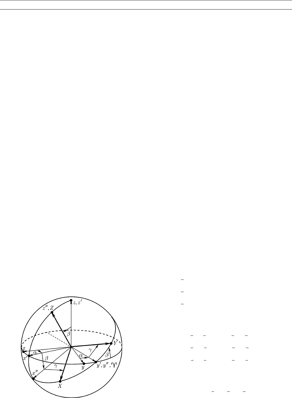
Euler a ngles ð a; b; g Þ

In this system the ðx ; y; zÞ reference frame is rotated through an angle a

about the z axis to form the ðx

; y

; z

Þ reference frame, which is

rotated though an angle b about the y

-axis to form the ð x

; y

; z

reference frame, which is rotated through an angle g about the

axis to form the final ðX ; Y ; Z Þ frame (see Figure H7). The point

with coordinates of r becomes a point with coordinates R in the rotated

reference frame, and the relationship can be written

R ¼ A ða ; b ; gÞ r; (Eq. 192)

where the matrix Aða; b; gÞ has the form

Aða; b; gÞ¼

cos a cos b cos g sin a cos b cos g sin b cos g

sin a sin g þcos a sin g

cos a cos b sin g sin a cos b sin g sin b sin g

sin a cos g þcos a cos g

cos a sin b sin a sin b cos b

(Eq. 193)

For the reverse rotation, the Euler angles ða; b; gÞ are replaced by

ðg; b; gÞ,

r ¼ Aðg; b; aÞR: (Eq. 194)

The matrix can be written in terms of its factors, which derive from the

three rotations:

cos g sin g 0

sin g cos g 0

001

cos b 0 sin b

01 0

sin b 0 cos b



cos a sin a 0

sin a cos a 0

001

(Eq. 195)

Comparing the off-diagonal terms of Að n ; V Þ of Eq. (147), and

A ð a; b; gÞ of Eq. (193), gives

sin a sin b ¼ cb ð1  cos VÞa sin V ;

sin b sin g ¼ cbð1  cos V Þþa sin V ;

sin b cos g ¼ cað1  cos VÞb sin V ;

cos a sin b ¼ acð1  cos VÞþb sin V ;

cos a cos b sin g 

sin a cos g ¼ abð1  cos VÞc sin V ;

sin a cos b cos g þ cos a sin g ¼ bað1  cos V Þþc sin V;

(Eq. 196)

and from Eq. (196) it follows that

a sin V ¼

sin bðsin g  sin aÞ;

b sin V ¼

sin bðcos g þ cos aÞ;

c sin V ¼

ð1 þ cos bÞsinðg þ aÞ: (Eq: 197)

The right-hand sides of Eq. (197) can be written as a product of two terms,

a sin V ¼ 2sin

b sin

ðg  aÞcos

b cos

ðg þ aÞ;

b sin V ¼ 2sin

b cos

ðg  aÞcos

b cos

ðg þ aÞ;

c sin V ¼ 2cos

b sin

ðg þ aÞcos

b cos

ðg þ aÞ; (Eq: 198)

from which we obtain

ða

þ b

Þsin

V ¼ 4 sin

b cos

ðg þ aÞ: (Eq. 199)

Comparing the diagonal terms of Að n; V Þ of Eq. (147), and A ða ; b ; gÞ

of Eq. (193), gives

Figure H7 The Oxyz reference frame is rotated through Euler

angles ða; b; gÞ to become the OXYZ reference frame.

HARMONICS, SPHERICAL 393

cos a cos b cos g  sin a sin g ¼ cos V þ a

ð1  cos V Þ;

 sin a cos b sin g þ cos a cos g ¼ cos V þ b

ð1  cos V Þ;

cos b ¼ cos V þ c

ð 1  cos V Þ;

(Eq. 200)

from the third of Eq. (200) we obtain

sin

b ¼ sin

V  c

sin

V ¼ða

þ b

Þ sin

V (Eq. 201)

From Eqs. (199) and (201)

cos

V ¼ cos

b cos

ðg þ a Þ;

and the positive square root is required, because in the case in which

a ¼ g ¼ 0, the angle of rotation V ¼ b. Therefore

cos

V ¼ cos

b cos

ð a þ gÞ: (Eq. 202)

Euler-Ro drigues param eters and Eu ler angles

Combining the results of Eq. (161) for rotation about n axis, with

Eqs. (198) and (202),

p ¼ a sin

V ¼ sin

b sin

ð g  aÞ;

q ¼ b sin

V ¼ sin

b cos

ð g  aÞ;

r ¼ c sin

V ¼ cos

b sin

ð g þ aÞ;

s ¼ cos

V ¼ cos

b cos

ð g þ a Þ; (Eq: 203)

and these important equations relate the axis and angle of rotation with

the Euler angle formulation of the same rotation.

Cayley- Klein param eters and E uler angles

Using the Cayley-Klein parameters, u,v, defined in Eq. (175), and the

results of Eq. (203),

u ¼ s þ i r ¼ cos

V þ i c sin

V ¼ cos

b e

i ðg þa Þ

;

v ¼ q þ i p ¼ðb þ i aÞ sin

V ¼ sin

b e

i ðg a Þ

: (Eq: 204)

In terms of the rotation matrix elements D

ða ; b ; gÞ , (see Spherical

harmonics ), and the generalized Legendre functions d

M ;m

ð bÞ , the para-

meters u and v are

u ¼ D



;

ða; b; gÞ¼d



;

ðbÞe

iðaþgÞ=2

;

v ¼ D

;

ða; b; gÞ¼d

;

ðbÞe

iðaþgÞ

: (Eq: 205)

Spherical harmonics

Briefly, spherical harmonics are multiple derivatives of inverse

distance,

ð1Þ

lm

]

]



]



lm

lþ1

ﬃﬃﬃﬃﬃﬃﬃﬃﬃﬃﬃﬃﬃﬃﬃﬃﬃﬃﬃﬃﬃﬃﬃﬃﬃﬃﬃﬃﬃﬃﬃﬃ

ðl þ mÞ!ðl  mÞ!

2l þ 1

ðy; fÞ:

(Eq. 206)

and on using the spinor forms of derivatives given in Eqs. (187)– (206),

it follows that solid spherical harmonics can also be written in a more

symmetric, spinor form,

lþ1

ðy; fÞ¼ð1Þ

lm

ﬃﬃﬃﬃﬃﬃﬃﬃﬃﬃﬃﬃﬃﬃﬃﬃﬃﬃﬃﬃﬃﬃﬃﬃﬃﬃﬃﬃﬃﬃﬃﬃ

2l þ 1

ðl  mÞ!ðl þ mÞ!

lm

lþm

(Eq. 207)

Using the transformation law (191) for spinors, under rotation of the

reference frame, the transformation law for spherical harmonics is

easily derived. This leads, for example, to formulae in spherical (and

hyperspherical) trigonometry, and to the identification of vector and

tensor quantities, which are formed into “irreducible” parts, with pro-

found physical implications, on account of their identification as sphe-

rical harmonics in their own right.

Denis Winch

Bibliography

Chapman, S., and Bartels, J., 1940. Geomagnetism. London: Oxford

Clarendon Press.

Condon, E.U., and Shortley, G.H., 1935. The Theory of Atomic Spec-

tra. Cambridge: Cambridge University Press. [7th printing 1967.]

Ferrers, Rev. N.M., 1897. An Elementary Treatise on Spherical Har-

monics and Subjects Connected with them. London: Macmillan

and Co.

Goldie, A.H.R., and Joyce, J.W., editors, 1940. Proceedings of the

1939. Washington Assembly of the Association of Terrestrial Mag-

netism and Electricity of the International Union of Geodesy and

Geophysics. International Union of Geodesy and Geophysics

(IUGG), Edinburgh: Neill & Co., Bulletin 11, part 6, 550.

Kendall, M.E., and Moran, P.A.P., 1962. Geometrical Probability.

London: Griffin.

Maxwell, J.C., 1881. A Treatise on Electricity and Magnetism. 2nd

edition. London: Oxford Clarendon Press.

Schendel, L., (1877). Zusatz zu der Abhandlung über Kugelfunktionen

S. 86 des 80. Bandes. Crelle’s Journal, 82: 158–164.

Schmidt, A., 1899. Formeln zur Transformation der Kugelfunktionen

bei linearer Änderung des Koordinatensystems.

Zeitschrift für

Mathematik, 44: 327–338.

Schuster, A., 1903. On some definite integrals, and a new method of

reducing a function of spherical coordinates to a series of spherical

harmonics. Philosophical Transactions of the Royal Society of

London, 200: 181–223.

Varshalovich, D.A., Moskalev, A.N., and Khersonskii, V.K., 1988.

Quantum Theory of Angular Momentum. Irreducible Tensors,

Spherical Harmonics, Vector Coupling Coefficients, 3nj Symbols.

Singapore: World Scientific Publishing Co.

Vilenkin, N.J., 1968. Special Functions and the Theory of Group

Representations, American Mathematical Society, Second printing

1978. Translated from 1965 Russian original by V.N. Singh.

Wigner, E., 1931. Gruppentheorie und ihre Anwendungen auf die

Quantenmechanik und Atomsspektren, Braunschweig. Translation:

Griffin, J.J. (ed.) (1959). Group Theory and its Application to the

Quantum Mechanics of Atomic Spectra. New York and London:

Academic Press.

Whittaker, E.T., 1904. Treatise on the Analytical Dynamics of Parti-

cles and Rigid Bodies. Cambridge: Cambridge University Press.

394 HARMONICS, SPHERICAL

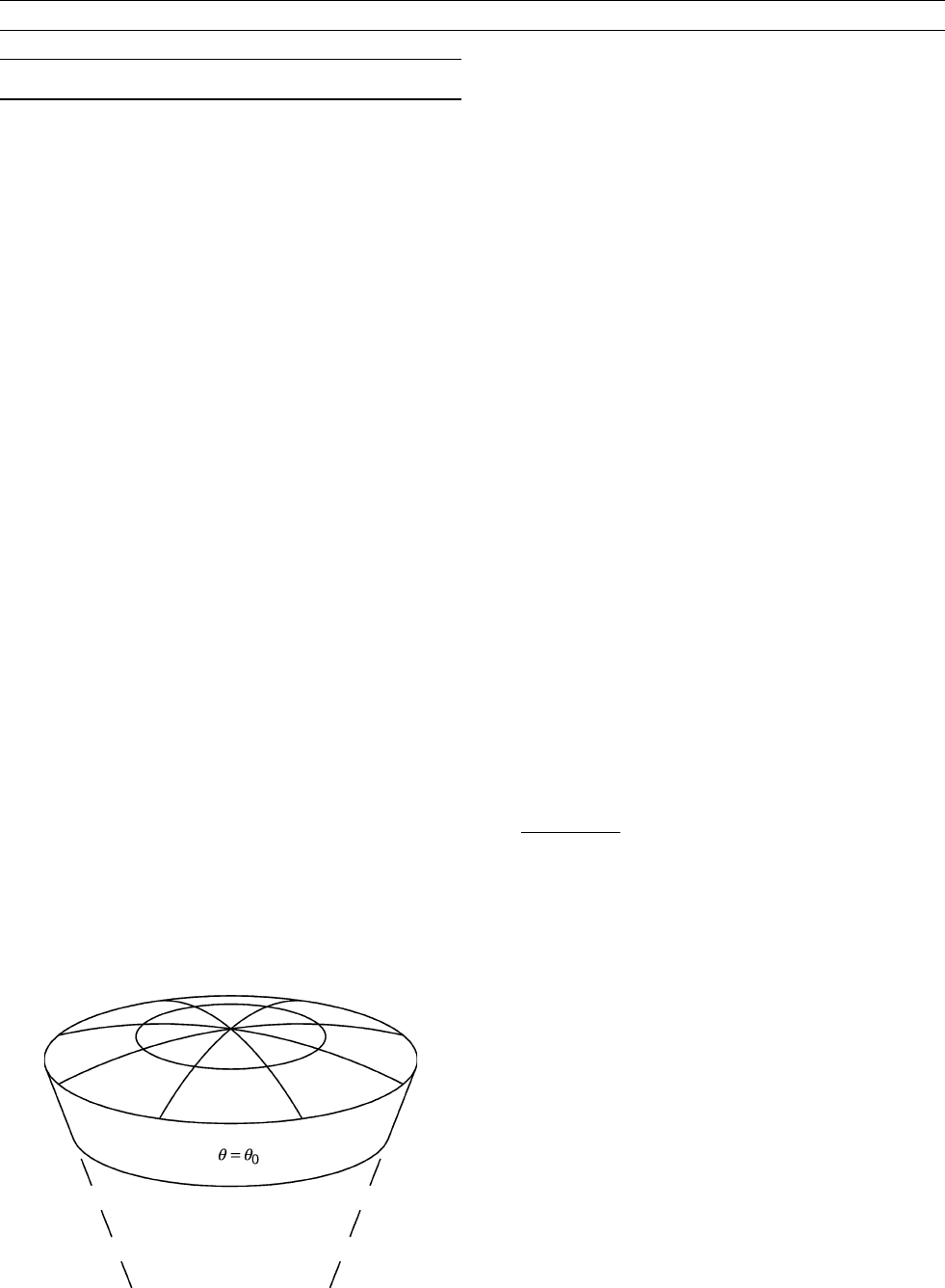
HARMONICS, SPHERICAL CAP

Spherical cap harmonics are used to model data over a small region of

the Earth, either becaus e data are only available over this region

or because interest is confined to this region. The three-d imensional

region considered in this article is that of a spherical cap (Figure H8),

although one can also consider only the two-dimensional surface

of a spherical cap. A three-dimensional model is used where the

data are vector data that represent a field with zero curl and diver-

gence, whereas a two-dimensional model is used for general fields

with no such constraints.

In a source free region of the Earth, the vector magnetic field B can

be expressed as the gradient of a scalar harmonic potential V. (This

scalar potential is “ harmonic” since its Laplacian is zero.) The poten-

tial, and therefore the field, can then be expressed mathematically as

a series of basis functions, each term of the series being harmonic by

design. This harmonic solution is usually identified by the coordinate

system used. For example, when the coordinates chosen are rectangu-

lar coordinates, we say the field is expressed in terms of rectangular

harmonics. These would be useful when dealing with a local or very

small portion of the Earth ’s surface, such as in mineral exploration.

When the coordinate system is the whole sphere, we speak of spherical

harmonics (see Harmonics, spherical ). These are used for investigat-

ing global features of the field. This article will discuss the harmonic

solution for the case of a spherical cap coordinate system, which

involves wavelengths intermediate between the local and the global

solutions.

Basis fu nction s

The basis functions for the series expansion of the potential over a

spherical cap region are found in the usual way by separat ing the vari-

ables in the given differential equations (that the curl and divergence

of the field are zero) and solving the individual eigenvalue problems

subject to the appropriate boundary conditions (e.g., Smythe, 1950;

Sections 5.12 and 5.14). The boundary conditions include continuity

in longitude, regularity at the spherical cap pole, and the appropriate

Sturm-Liouville conditions on the basis functions and their derivatives

at the boundary of the cap (e.g., Davis, 1963, Section 2.4). The details

have been given by Haines (1985a), and computer programs in Fortran

by Haines (1988).

Let r denote the radius, y the colatitude, and l the east longitude of

a given spherical cap coordinate. This coordinate system is, of course,

identical to the usual spherical or polar coordinate system, except that

the colatitude y must be less than y

, the half angle of the spherical cap

(Figure H8). Also, the spherical cap pole is not usually the geographic

North Pole, in which case the geographic coordinate system is rotated

to the new spherical cap pole giving new spherical cap colatitudes and

longitudes. In both spherical and spherical cap systems, the radius r

must lie between the outer radius of any current sources within the

Earth and the inner radius of any current sources within the iono-

sphere, and the longitude l takes on the full 360



range. The harmonic

solution of the potential V ð r ; y; lÞ applicable to this three-dimensional

spherical cap region is then given by:

V ðr ; y ; l Þ¼ a

k ¼ 0

m¼ 0

ða = r Þ

ð mÞþ 1

ðmÞ

ð cos y Þ

½g

m; i

cosð ml Þþh

m;i

sin ð ml Þ

þ a

k ¼ 1

m¼ 0

ð r = a Þ

ðmÞ

ð mÞ

ðcos y Þ

½g

m; e

cos ðm lÞþ h

m; e

sin ðm l Þð Eq: 1Þ

where a is some reference radius, usually taken as the radius of the

Earth, and P

ð mÞ

ðcos y Þ is the associated Legendre function of the

first kind. It is usual in geomagnetism for the Legendre functions P to

be Schmidt-normalized (Chapman and Bartels, 1940; Sections 17.3

and 17.4). The subscript of P is known as the degree of the Legendre

function and the superscript is known as the order; k is referred to as

the index and simply orders the real (usually nonintegral) degrees

ð mÞ . The g

and h

are the coefficients, which are each further identi-

fied with the superscript i or e to denote internal or external sources,

respectively. The internal source terms involve powers of ( a/ r) while

the external source terms involve powers of (r /a ). If one intended to fit

only internal (or external) sources, only the internal (or external) terms

of the expansion would be used. The truncation indices K

and K

are

the maximum indices for the internal and external series, respectively.

The potential can easily be transformed into a function of time t as

well as space, V ðr ; y ; l ; t Þ , by simply making the coefficients functions

of time, g

ð t Þ and h

ðt Þ , and expanding these coefficients in terms of

some temporal basis functions, such as cosine functions or Fourier

functions or whatever is appropriate.

The degree n

ð mÞ is chosen so that

ð mÞ

ðcos y

d y

¼ 0 when k  m ¼ even (Eq. 2)

and

ðmÞ

ð cos y

Þ¼ 0 when k  m ¼ odd (Eq. 3)

where the Legendre functions P

ð cos y

Þ are here considered to be

functions of n , given the order m and the cap half-angle y

. The index

k simply starts at m and is incremented by 1 each time a root is found

to one of the Eqs. (2) or (3). This choice of k is analogous to the

case of ordinary spherical harmonics (y

¼ 180



), and in fact for that

case the degree n

(m) is simply the integer k. Table H3 gives the roots

ð mÞ for y

¼ 30



,upto k ¼ 8. Figure H9 shows how P

ðmÞ

ð cos yÞ

varies over a 30



cap, up to index 4, both for k  m ¼ even and for

k  m ¼ odd.

We can see how the P

ð mÞ

ð cosy Þ,0 y  y

, for k  m ¼ even,

are analogous to the cosine functions cos ð ny Þ,0 y  p, in that each

has zero slope at the upper boundary (y

or p, respectively). In fact, we

can think of P

ðmÞ

as being defined on the interval ½ y

;þy

, just

as cosðnyÞ is defined on ½p; þp, so that an expansion over the

spherical cap using P

ðmÞ

ðcosyÞ, k  m ¼ even, as basis functions is

analogous to an expansion in Cartesian coordinates over ½p; þp

using cos ðnyÞ as basis functions. The extension of P

ðmÞ

to the

½y

; 0 interval of course, takes place on the meridian 180



away

from the meridian on which the ½0; þy

 interval lies, which is why

the P

ðmÞ

ðcosyÞ must be zero at y ¼ 0 when m 6¼ 0(Figure H9a).

Figure H8 Three-dimen sional spherical cap region: colatitude

y  y

. Thickness of cap indicates radial coverage of data.

HARMONICS, SPHERICAL CAP 395