Gubbins D., Herrero-Bervera E. Encyclopedia of Geomagnetism and Paleomagnetism

Подождите немного. Документ загружается.

of the sample is provided by an electromagnet, or superconducting sole-

noid if fields greater than 3T are required. A heater or cryostat can be

fitted for variable temperature measurements.

VSMs are usually at least an order of magnitude less sensitive than

AGMs but have the advantage of being able to handle much larger

sample sizes (Lindemuth et al., 2000), and are thus more suitable for

standard paleomagnetic samples. The VSM, like the AGM, is gener-

ally used for high-field measurements, such as hysteresis properties.

The large metal poles of the DC electromagnets used to generate the

uniform field will have a residual field even when no current flows

through the coils (the residual remanence of the pole pieces is avoided

by using a field-controlled (with Hall sensor) power supply). The dif-

ficulty in reducing the ambient field in the region of the sample to a

sufficiently low value makes these instruments unsuitable for low field

(remanence) measurements.

Translation balance

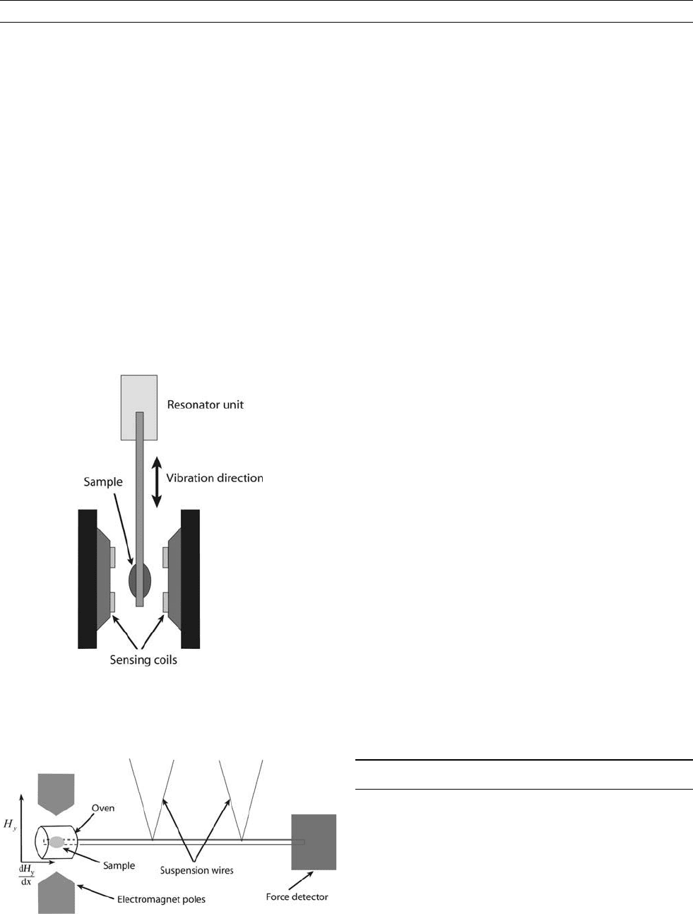
A translation balance in its simplest form consists of a rod suspended

by wires so it is free to make small movements along its axis (see

Figure M157). The sample is placed at one end of the rod, and a field

is created perpendicular to the rod axis, by means of a large electro-

magnet. The field produced by the electromagnet will have a gradient

along the rod axis, and the force on the magnetic sample will therefore

be given by F ¼ M dH

/dx, where M is the sample magnetization (see-

Figure M157). This force causes a translation of the rod, which is cali-

brated against the samples magnetization. Such instruments will

normally have an oven surrounding the sample so that the magnetiza-

tion can be measured as a function of temperature, allowing the Curie

point to be determined. Sensitivities of 10

–9

can be achieved

with these instruments.

Cryogenic magnetometers

SQUID magnetometers (described above) are also used in magnetic

mineralogy. Here, the requirement for liquid helium to keep the sen-

sing coils superconducting can also be used to cool the sample, and

provide large fields (greater than 5T) in superconducting solenoids.

It is therefore possible to measure over a wide range of temperatures

(down to less than 2K) and fields. However SQUID sensors do not

allow continuous measurement of magnetization versus field strength.

To change the field within a superconducting coil it must be switched

out of its superconducting state. This requirement makes field depen-

dency observations much more time consuming compared to similar

measurements on a VSM or AGM.

Wyn Williams

Bibliography

Blackett, P.M.S., 1952. A negative experiment relating to magnetism

and the Earth’s rotation. Philosophical Transactions of the Royal

Society of London, Series A, 245: 309–370.

Collinson D.W., 1983. Methods in rock magnetism and palaeomagnet-

ism. Techniques and Instrumentation. London: Chapman & Hall.

O’Grady, K., Lewis V.G., and Dickson D.P.E., 1993. Alternating gra-

dient force magnetometry: applications and extension to low tem-

peratures. Journal of Applied Physics , 73: 5608–5613.

Lindemuth, J., Krause J., and Dodrill B., 2000. Finite sample size

effects on the calibration of vibrating sample magnetometer. IEEE

Transactions on Magnetics, 37: 2752–2754.

Cross-references

Compass

Gauss’ Determination of Absolute Intensity

Instrumentation, History of

Observatories, Automation

Observatories, Instrumentation

Rock Magnetometer, Superconducting

MAGNETOSPHERE OF THE EARTH

The Earth’s magnetosphere is the region surrounding the planet, above

the outer atmosphere and ionosphere (q.v.), which contains and is con-

trolled by the Earth’s magnetic field. It extends from an altitude of

500 km above the Earth’s surface to an outer boundary which is

formed by the interaction of the planetary magnetic field with the solar

wind, the plasma (charged particle) gas that streams continuously

outward from the Sun. On the dayside, the compressive effect of the

solar wind confines the field to a region extending 10 Earth radii

from the Earth, while on the nightside the field is stretched into a long

comet-like tail which extends typically in excess of 1000 Earth radii.

The Earth’s radius, R

6400 km, is thus a convenient measure of mag-

netospheric spatial scales. Electric currents flowing in these regions,

whose magnetic effects can be observed at the Earth’s surface, include

Figure M156 A schematic of a vibrating sample magnetometer.

The sample is vibrated mechanically, and the induced signal in

the sensing coils will be proportional to its magnetization.

Figure M157 The principle elements of a horizontal translation

balance. An electromagnet produces a large magnetizing field

along the y-axis and a field gradient along the x-axis that

generates a force on the sample proportional to its magnetization.

656 MAGNETOSPHERE OF THE EARTH

those flowing at the solar wind-magnetosphere boundary, those produced

by the drift of energetic charged particles inside the magnetosphere, and

those associated with the coupling between the magnetosphere and the

ionosphere Ohtani et al. (2000). Magnetic perturbations observed at the

Earth’s surface due to these three sources peak typically at a few tens, a

few hundreds, and a few thousands of nanoteslas, respectively , and vary

on a range of timescales from minutes to hours and days. In this article

we first concentrate on theoverall structure and basic physics of the coupled

solar wind-magnetosphere-ionosphere system, and then consider the

dynamic processes which occur, leading to strong temporal variations.

Structure of the magnetosphere

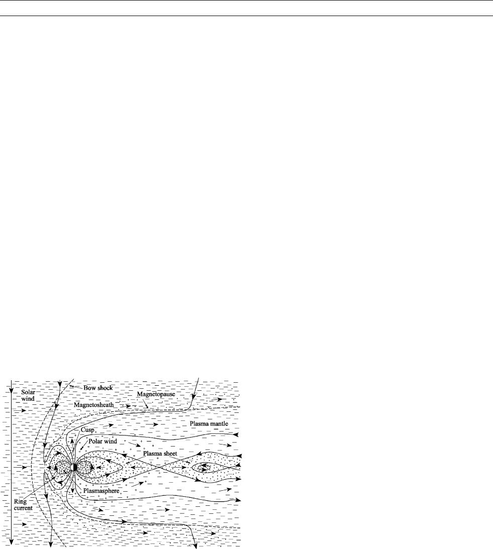
In Figure M158 we show a cross-section through the Earth’s magneto-

sphere in the noon-midnight meridian plane, where the arrowed solid

lines indicate magnetic field lines. The small symbols indicate the

main plasma populations, while the arrows show their principal flows.

The small dashes show the solar wind plasma, together with the mag-

netospheric “boundary layer” plasma populations derived directly from

it. The direction of the Sun is toward the left, so that the solar wind

flows from left to right as indicated. The solar wind derives from

hydrogen gas in the solar atmosphere, which is heated sufficiently

strongly in the solar corona, to temperatures in excess of a million

degrees, that the atoms are fully broken up by collisions to form a

plasma of electrons and protons (plus a few percent a-particles from

helium), which then streams continuously out into the solar system

at speeds 500 km s

1

. At the orbit of the Earth, the proton and elec-

tron number densities are 10 cm

–3

, sufficiently low that the particles

in the gas are collision-free, meaning that the mean free path for parti-

cle collisions is comparable with or larger than the size of the

system. A second source of plasma in the magnetosphere derives from

the Earth’s upper atmosphere, which is relatively cool (1000 K)

but is partially ionized by solar far-UV and X-rays at altitudes above

100 km, forming the ionosphere. These charged particles, consisting

of protons and heavy ions, principally singly-charged oxygen, together

with corresponding electrons, can also stream out of the topside iono-

sphere into the magnetosphere, as indicated by the small crosses in the

figure. In the ionosphere, collisions between ions and neutral atoms are

significant at altitudes up to 500 km. Above this altitude, however,

the ionospheric ions also become collision-free due to falling densities,

500 km thus being chosen (rather arbitrarily) above as the “base” of

the magnetosphere, where it interfaces with the ionosphere. Like the

solar wind, therefore, the plasma of charged particles in the Earth’s

magnetosphere is also collision-free. Although the Earth’s neutral

atmosphere is detectable throughout the magnetosphere to distances

of at least 10 R

(forming a hydrogen “geocorona” originating from

the photodissociation of water vapor lower in the atmosphere), the

behavior of neutral and charged particle populations within it are

largely decoupled due to the lack of collisions, apart from the occa-

sional charge-exchange reaction between them.

When collisions can be ignored, the motion of ions and electrons in

the plasma is governed by the forces of the large-scale fields prevail-

ing, and for both solar wind and magnetosphere the most important

forces by far are electromagnetic. Solar and planetary gravity is only

important in the regions close to the bodies concerned, i.e., in the solar

corona near the Sun, and in the ionosphere near the Earth. The motion

of charged particles in a large-scale electromagnetic field consists of a

number of components, which take place on generally widely sepa-

rated timescales. The first is a rapid gyration of the particles around

the magnetic field lines in nearly circular orbits whose radius is gener-

ally tiny compared with the scale size of the systems. The second is a

uniform motion along the magnetic field lines, which is subject to the

magnetic mirror force which repels particles from regions of increasing

field strength along the field lines (i.e., is directed away from regions

where field lines converge). The mirror force is produced by the action

of the field strength gradient on the magnetic dipole formed by the

gyrating particle. In the quasidipolar field of a planetary magneto-

sphere, for example, the field strength along a given field line is

weakest at the equator and increases greatly toward the planet (see

Figure M158). This configuration can therefore trap charged particles

almost indefinitely, the mirror force resulting in a bounce motion

between mirror points in the northern and southern hemisphere. Only

those particles that are directed almost along the field lines at the

equator, which thus have small magnetic moments, can reach down

to the upper layers of the atmosphere. The third motion consists of

large-scale plasma flows transverse to the magnetic field lines, such

as that shown for the solar wind in Figure M158. Such flows are

associated with an electric field E directed transverse to the magnetic

field B, related to the plasma velocity V by the vector relation

E ¼V B. (The effect of additional cross-field drifts associated

with magnetic field inhomogeneity will be discussed further below.)

Inspection of the flows indicated in Figure M158 shows that the elec-

tric field is directed everywhere out of the plane of the diagram,

though it is not everywhere of equal strength. In such “crossed” elec-

tric and magnetic fields, charged particles drift perpendicular to the

magnetic field with velocity V ¼ E  BðÞ=B

independent of their

charge or mass, this expression being exactly equivalent to the vector

relation for E given above.

This “E  B drift” has a very special property, first discovered by

Alfvén in 1942 (see Alfvén’s theorem), that particles whose centers

of gyration lie initially on the same field line as each other, remain

on the same field line as each other for all time, thus showing why

plasma structures are strongly organized by magnetic field lines, as

indicated by various features in Figure M158. We may picture the col-

lective behavior as one in which the magnetic field and the plasma are

“frozen” together. However, we can think either of the plasma as mov-

ing and carrying the field lines, or equivalently of the field lines as

moving and carrying the plasma. Which of these pictures is the most

appropriate for a given system depends upon the relative energies in

the plasma and magnetic field. Thus, for example, since the plasma

Figure M158 Sketch of a cross section through the Earth’s

magnetosphere in the noon-midnight meridian plane. The

direction of the Sun is toward the left, such that the solar wind blows

from left to right. The arrowed solid lines show magnetic field lines,

while the heavy dashed lines show locations of principal field and

plasma discontinuities at the bow shock and magnetopause. The

small symbols indicate the principal plasma populations present,

while the arrows indicate their direction of flow. The dashes

indicate the solar wind, and the plasma populations derived directly

from it in the magnetosheath and magnetosphere (cusp and plasma

mantle). The crosses indicate plasma originating from the Earth’s

ionosphere (plasmasphere and polar wind), while the dots indicate

the heated plasma of mixed origin that originates in the tail (plasma

sheet and ring current).

MAGNETOSPHERE OF THE EARTH 657

energy exceeds the magnetic energy in the solar wind, the solar mag-

netic field is carried outward “frozen” into the expanding plasma flow,

forming a large-scale interplanetary magnetic field (IMF) that pervades

the entire solar system (see Figure M158). The strength of the IMF at

the Earth’s orbit is typically 5–10 nT, directed, on the average, in the

ecliptic plane at an angle of 45



to the Earth-Sun line. The latter tilt

is due to the rotation of the Sun, which winds the IMF into a spiral

form as the field lines are carried out into the solar system by the

plasma flow. On the other hand, in the quasidipolar field regions of

the magnetosphere and ionosphere, where the magnetic energy domi-

nates, we instead think of the field lines as moving, transporting the

plasma.

We may apply this “frozen-in” concept to the interaction between

the solar wind and the planetary magnetic field. Since the solar wind

and IMF are frozen together, as well as the planetary field and plane-

tary plasma (e.g., from the ionosphere), then when these two media

interact they will not mix. Instead, the solar wind confines the plane-

tary field to a cavity surrounding the planet, around which it flows,

as first deduced by Chapman and Ferraro in 1931 (see Chapman, Syd-

ney). This magnetic cavity is the planet’s magnetosphere, whose outer

boundary, shown by the dashed line in Figure M158 , is called the

“magnetopause.” A “bow shock” forms ahead of the cavity, also

shown by a dashed line in Figure M158, due to the fact that the mag-

netosphere represents a blunt obstacle in the supersonic solar wind

flow. Across the shock the solar wind is slowed, compressed, and

heated, forming the turbulent “magnetosheath” layer located between

the shock and the magnetopause boundary.

The size of the magnetospheric cavity is set by the condition of

pressure balance at the boundary. A simple estimate of the distance

of the equatorial boundary at noon (the minimum distance in the direc-

tion facing the Sun) can be made by equating the ram pressure of the

solar wind on one side of the boundary, with the magnetic pressure

=2m

) of the compressed planetary field on the other. With typical

solar wind values the radial distance of the boundary is estimated to

be 10 R

on this basis, as observed, a position which may vary by

factors of up to two in either direction under extreme solar wind

conditions. The strength of the compressed planetary field just inside

the boundary is typically 60 nT, representing a planetary dipole

field of 30 nT enhanced by a factor of 2 by the electric current

flowing in the magnetopause boundary. This latter current is termed

the “Chapman-Ferraro” current, and inspection of Figure M158 with

Ampere’s law in mind shows that it flows out of the plane of the dia-

gram in the equatorial region on the dayside, closing over the magne-

topause into the plane of the diagram over the polar regions and on the

nightside. These rings of magnetopause current produce a perturbation

magnetic field in the near-Earth magnetosphere whose strength is typi-

cally a few tens of nanoteslas directed northward (i.e., upward in

Figure M158), hence enhancing the horizontal field at low and middle

latitudes at the Earth’s surface.

Frozen-in behavior of the field and plasma associated with the

E  B drift is not, however, a universally valid description. In a colli-

sion-free medium it is broken in particular by the presence of addi-

tional particle drifts, the most significant of which cause ions and

electrons to drift in opposite directions across the field (thus producing

a current) due to the presence of gradients in the strength and direction

of the magnetic field. These “field inhomogeneity” drifts are propor-

tional to the field gradients, and also to the particle energy, thus being

more important for particles of higher energy. When the field gradients

are weak, these additional drifts are important only for particles in the

high-energy tail of the energy distribution, and frozen-in motion then

represents a useful organizing concept for the bulk of the plasma popu-

lation. This limit applies essentially throughout the solar wind, and

through most of the Earth’s magnetosphere. However, when the field

gradients are very strong, such that the motion of the bulk of the

plasma particles is affected, then the frozen-in picture breaks down.

One such place where this happens is the magnetopause boundary,

where the field strength and direction in general switch rapidly from

magnetosheath to magnetosphere values across the magnetopause cur-

rent sheet. The simplest theoretical description of the consequence of

frozen-flux breakdown is that the magnetic field diffuses through the

plasma, locally, in the region of the strong gradient. As first pointed

out by Dungey in 1961, this then allows magnetic field lines to

become joined across the boundary, producing “open” magnetic field

lines which pass from the solar wind at one end, through the magneto-

pause, to the Earth ’s polar regions at the other. This process is called

“magnetic reconnection.” Two newly reconnected open field lines are

shown in Figure M158 passing through the dayside magnetopause

shortly after reconnection has taken place near the equator. Sharply

bent magnetic field lines exert a tension force on the plasma like the

force of rubber bands (the force per unit volume being j  B, where

j is the current density in the plasma), in this case accelerating the

boundary plasma poleward away from the equator, such that the field

lines also contract poleward, releasing energy to the plasma and allowing

further reconnection to proceed at the equator. Subsequently, the open

field lines are carried downstream frozen into the magnetosheath

flow, and are stretched out into a long cylindrical comet-like tail. This tail

consists of two lobes, D-shaped in cross-section, one connected to the

northern polar region at Earth, the other to the southern, as indicated in

Figure M158. Observations show that the tail lobe field lines remain

open typically for a few hours, such that with a downstream speed of

500 km s

–1

, the tail is typically 1000 R

long.

The open field lines form magnetic pathways along which the

magnetosheath plasma may enter the magnetosphere. Such plasma

thus flows along newly opened field lines to form a boundary layer

adjacent to the dayside magnetopause, and the “cusp” population as

it then moves down toward the Earth (see the magnetospheric dashed

regions in Figure M158). The majority of the particles, however, are

repelled by the magnetic mirror force as the field strength increases

near the Earth, and hence move back out again toward the outer mag-

netosphere. Due to the antisunward motion of the open field lines,

however, the cusp plasma flows back out into the lobes of the tail,

in the region adjacent to the magnetopause, forming the “plasma man-

tle” population. As the open field lines are carried down the tail, so the

field lines and mantle plasma sink in toward the center plane of the

tail, followed by further entry of antisunward flowing magnetosheath

plasma at the tail magnetopause, such that the mantle grows wider

and with increasing density at larger distances. Plasma from the

Earth’s polar ionosphere also flows into the lobes (cross symbols

in Figure M158), but because of its low velocity along the field lines

(10 km s

1

), it does not reach far down the tail on the few-hour time-

scale that the lobe field lines remain open. Overall, the plasma density

in the inner part of the tail lobes is very low, 0.01–0.1 cm

–3

, and with

temperatures typically of order a few tens to a few hundred electron-

volts, most of the system energy resides in the lobe magnetic field.

(Note that while temperatures in the solar and terrestrial ionized atmo-

spheres are generally quoted in Kelvin, as above, the temperatures of

magnetospheric plasmas are usually indicated by the mean or typical

energy of the particles W, in eV. To convert between them, we note

that for a near-Maxwellian velocity distribution T KðÞ10

W eVðÞ.

Thus, for example, typical hot magnetospheric plasma of 1 keV mean

energy corresponds to a temperature of 10

K.)

The residency of the oppositely directed open field lines in the two

tail lobes is terminated when they sink into the center plane of the tail

and reconnect in the equatorial current sheet that separates them, as

shown by the X-shaped field configuration on the right side of

Figure M158. On the tailward side of the tail reconnection site the

lobe field lines become disconnected from the Earth, and the j  B

(rubber band) tension force accelerates the tail plasma rapidly away

from the Earth, where it eventually rejoins the solar wind. On the

Earthward side, the process forms new “closed” field lines, connected

to the Earth at both ends, which similarly contract rapidly earthward,

compressing and heating the lobe plasma as they do so. This hot

plasma, containing both solar wind and ionospheric contributions, is

termed the “plasma sheet” population, and is shown by the dotted

658 MAGNETOSPHERE OF THE EARTH

region in Figure M158. In the near-Earth tail it is characterized by

densities 0.1–1cm

–3

, and electron and ion temperatures of 0.5

and 5 keV, respectively, but both density and temperatures increase

as the plasma flows earthward into the quasidipolar inner magneto-

sphere and is further compressed and heated. Throughout these regions

the hot plasma sheet population carries a current, due to the field-

inhomogeneity effects mentioned above, which is directed westward,

i.e., out of the plane of Figure M158 on the nightside of the Earth,

and into the plane of the diagram on the dayside. On the nightside

within the tail, the current paths reach the tail boundary, and close over

the magnetopause to form two D-shaped solenoids lying back-to-back,

as required by the lobe magnetic field structure. Nearer the Earth, the

current paths may close wholly round the Earth to form a plasma “ring

current” (q.v.). Overall, these currents produce a perturbation field at

the Earth, which is directed southward (i.e., downward in Figure

M158), and is usually a few tens of nanoteslas in amplitude. However,

as we discuss below, these currents become greatly enhanced during

magnetic storms (q.v.), producing perturbation fields up to an order

of magnitude larger.

The closed field lines and hot plasma produced in the tail subse-

quently flow sunward around the Earth in the quasidipolar magneto-

sphere, eventually reaching the dayside magnetopause where they

become open again, allowing the hot magnetospheric plasma to escape

into the magnetosheath, as indicated by the dotted region outside the

magnetopause. Overall, therefore, reconnection at the magnetopause

and in the tail results in the formation of a large-scale cyclical flow

of field lines and plasma through the Earth’s magnetosphere, first dis-

cussed by Dungey in 1961. The overall cycle time is 12 h, of which

the field lines spend 4 h open in the tail lobes, and 8 h closed flow-

ing sunward through the central magnetosphere. The solar wind is not,

however, the only source of momentum that drives magnetospheric

flow. A second source resides in the rotation of the Earth, and the

coupled rotation of the Earth’s upper atmosphere. Collisions between

ions and neutral atmospheric particles in the ionosphere produce a fric-

tional force on the feet of the magnetospheric field lines which tends to

spin them up toward rotation with the planet, a flow called “corota-

tion.” In general, the overall magnetospheric flow results from a sum-

mation of the effects of the planetary and solar wind driving forces.

The corotation effect tends to produce a flow in the equatorial plane

increasing linearly with the distance from the planet (i.e., a flow with

the planetary angular velocity), while in the simplest picture of a

dipole magnetic field and uniform cross-system electric field, the

equatorial Dungey-cycle flow increases as the cube of the distance

(i.e., as the inverse of the field strength). Reflection on these relative

dependencies then shows that corotation will dominate close-in, and

Dungey-cycle convection at larger distances. For Earth, the boundary

between these flow regimes is located typically at 5 R

in the equa-

torial plane, about half-way to the dayside magnetopause. The hot

plasma flowing in from the tail is therefore excluded from this inner

core of corotating field lines, as indicated in Figure M158, which

is instead filled to relatively high densities (100–1000 cm

–3

)by

cold (1–10 eV) hydrogen and oxygen plasma from the ionosphere.

This population is termed the plasmasphere, and is indicated by the

near-Earth region of dense crosses in Figure M158.

Magnetosphere-ionosphere coupling

The magnetospheric flows discussed above produce corresponding

motions of the field and plasma in the polar ionosphere, resulting

in large-scale current systems flowing between these regions.

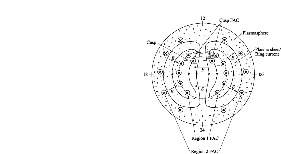
Figure M159 shows a view looking down on the North Polar Region,

with noon (the direction toward the Sun) at the top of the diagram,

dusk to the left, dawn to the right, and midnight at the bottom. The

central circular dashed line shows the outer boundary of the “open”

field region (located typically at magnetic latitudes of 75



at noon

and 70



at midnight), while the arrowed solid lines show plasma

streamlines. The open field lines within the dashed line boundary,

mapping to the northern tail lobe, flow antisunward from noon to mid-

night at speeds typically of a few 100 m s

–1

, while the closed field

lines at lower latitudes return sunward. This twin-vortex flow is the

signature of the Dungey-cycle in the ionosphere. The  V  B elec-

tric field associated with the flow is directed from dawn to dusk across

the open field line region as indicated, reversing in sense to poleward

at dusk and equatorward at dawn. The small symbols also show the

magnetospheric plasma populations into which the ionospheric field

lines map, the symbol code corresponding to that in Figure M158. Ions

and electrons from the cusp (dashes) and plasma sheet (dots) precipi-

tate into the upper atmosphere, excite the atoms (typically at altitudes

100–300 km), and cause them to emit photons, giving rise to one

component of auroral light emissions (see Auroral oval) Paschmann

et al. (2002) and Sandholt et al. (2001). They also ionize the neutral

atoms and increase the plasma density of the ionosphere, a process that

is especially important at night when the solar production mechanism

is inoperative.

The Dungey-cycle flow drives two components of electric current in

the lower ionosphere, both resulting from the effects of collisions

between ionospheric ions and atmospheric neutral particles. At alti-

tudes below 120 km, these collisions become sufficiently frequent

that the ions do not move with the field lines at all, but are essentially

tied to the generally smaller motions of the upper atmosphere (i.e., the

winds in the neutral thermosphere). However, the electron motion

remains almost unaffected by collisions, frozen to the field line motion

Figure M159 Sketch looking down onto the northern polar

ionosphere, with noon (the direction toward the Sun) at the top of

the diagram, dusk to the left, dawn to the right, and midnight at

the bottom. The dashed line shows the boundary between open

and closed magnetic field lines, while the arrowed solid lines

show the streamlines of the Dungey-cycle plasma flow driven by

solar wind-magnetosphere interaction. The short arrows marked

E indicate the directions of the electric field associated with the

flow, E ¼V  B (the magnetic field points into the northern

ionosphere), while the circled dots and crosses indicate regions

of upward and downward field-aligned current (FAC) flow,

respectively. The small symbols indicate the principal plasma

regimes into which the field lines map in the magnetosphere, with

the same format as Figure M158.

MAGNETOSPHERE OF THE EARTH 659

throughout the ionosphere, to altitudes below 100 km. Consequently,

in the layer between 100 and 120 km, ionospheric electrons flow

around the streamlines shown in Figure M159, carrying a current in

the opposite direction, while the ions in the layer remain almost

motionless, tied to the neutral atmosphere. This current, directed trans-

verse to both the electric and magnetic fields is thus termed a Hall cur-

rent, and with a height-integrated ionospheric conductivity of 10 mho

and typical ionospheric flows of several hundred meters per second, it

produces equal and opposite magnetic perturbations on either side of

the ionospheric Hall layer which are typically 100–200 nT in

strength. At the Earth’s surface in the northern hemisphere these per-

turbation fields are roughly in the direction of the overhead iono-

spheric electric field (opposite in the southern hemisphere). These

currents are nondissipative (i.e., j  E ¼ 0), and in principle can close

wholly within the ionosphere (for uniform conductivity), flowing

round the plasma flow streamlines.

The second current component flows at a slightly higher altitude of

120–150 km, where the ion motion is affected by collisions with

neutrals, but is not yet wholly dominated by them. In this layer colli-

sions provide the ions with some mobility in the direction of the elec-

tric field, while continuing to move approximately with the electrons

along the plasma streamlines. An ion current thus flows in the direc-

tion of E, termed the Pedersen current, and its magnitude is such that

the j  B force of the current, directed along the plasma streamlines,

just balances the frictional drag on the ionospheric plasma due to

ion-neutral collisions in the ionosphere. A key fact about the Pedersen

current is that it cannot, in principle, close within the ionosphere itself,

but is instead part of a large-scale current system which flows between

the magnetosphere and ionosphere, which imposes the flow of the for-

mer onto the latter in the presence of ionospheric ion-neutral drag. It

can be seen in Figure M159, for example, that the Pedersen currents,

directed along E, flow away from the open-closed field line boundary

on both sides at dawn, while flowing toward the boundary from both

sides at dusk. Current continuity then requires the presence of field-

aligned currents (FACs), which flow down the field lines from the

magnetosphere to the ionosphere at the dawn boundary, and up the

field lines from the ionosphere to the magnetosphere at the dusk

boundary. These are called the “region 1” FACs, whose direction is

indicated in Figure M159 by the circled dots and crosses for upward

and downward currents, respectively. These FACs close across the

field lines at large distances in the plasma which is the source of the

momentum producing the flow, i.e., in the magnetosheath plasma at

the tail magnetopause. The magnetic perturbations produced by the

overall current circuit bends the magnetic field lines in such a way that

the j  B force slows the magnetosheath plasma, while transferring the

momentum to the ionosphere to maintain the flow against collisional

frictional drag. Overall, this current system is solenoidal in nature,

such that the main magnetic effects are contained within the effective

current solenoid between the ionosphere and magnetopause. Thus

although the ionospheric height-integrated Pedersen conductivity is

generally comparable with the height-integrated Hall conductivity,

such that the two height-integrated current components are of similar

intensity in the ionosphere, the combined contribution of the iono-

spheric Pedersen current and the associated FACs approximately can-

cels underneath the ionosphere, and produces a much weaker

magnetic perturbation on the ground than that of the Hall current.

Above the ionospheric Pedersen layer, however, the perturbation field

produced by the Pedersen-FAC system is directed approximately

opposite to the plasma streamlines in the northern hemisphere, and

along the streamlines in the southern hemisphere. Typical amplitudes

in the region just above the Pedersen layer are again a few 100 nT.

The total current flowing in the “region 1” FAC system is typically

2–3 MA.

We also note from Figure M159 that Pedersen current continuity at

the equatorward boundary of the Dungey-cycle flow (typically located

at magnetic latitudes of 70



at noon and 65



at midnight), also

requires the presence of upward FACs at dawn and downward FACs

at dusk. These are called the “region 2” FAC system, in which the

upward currents at dawn close in the downward currents at dusk via

field-perpendicular currents flowing westward in the inner edge of

the equatorial plasma sheet population in the nightside magnetosphere

(and then via ionospheric Pedersen currents, the “region 1” FAC, and

the tail magnetopause). The total current flowing in the “region 2”

FACs is a little less than that in the “region 1” FACs, due to the fact

that the latter currents are fed by Pedersen currents from both open

and closed field line regions. We also note that regions of upward-

directed FAC are often associated with bright “discrete” auroras

(e.g., structured curtain-like forms), thus forming another component

of the auroral emissions. This is because upward currents are carried

primarily by warm plasma sheet electrons, which flow down the field

lines into the ionosphere. In order to produce a downward electron

flux which is sufficient to carry the upward current, the electrons

may be accelerated downward by an electric field directed upward

along the field lines (this being another scenario in which the frozen-

in picture breaks down). Typically the required field-aligned voltages

are a few kilovolts, such that the precipitating electrons carry a

sufficient energy flux to produce a bright aurora.

Magnetosphere dynamics

The above discussion has centered on the plasma physics principles

which govern the structure and properties of the coupled magneto-

sphere-ionosphere system, focusing particularly on the nature of the

current systems that flow within it. For clarity of exposition we have

viewed the system as being steadily driven, principally by the solar

wind, but also by planetary rotation. However, it is now important to

emphasize that the Earth’s plasma environment is almost never in such

a steady state, but generally varies strongly with time Cowley et al.

(2003). There are two reasons for this. The first is that the interplane-

tary medium which impinges on the Earth’s field itself varies strongly

with time, on timescales from a few minutes to the 27-day rotation

period of the Sun. There are also variations over the 11-year period

of the solar cycle. The second factor is that even when the solar wind

is relatively steady, the processes in the key interaction regions at the

magnetopause and in the tail show a propensity for pulsed behavior. We

will now outline these behaviors, beginning here with those which are

driven essentially directly by variations in the interplanetary medium.

Although the density and velocity of the solar wind determine the

size of the magnetospheric cavity and the speed with which open flux

tubes are transported to the tail, by far the most important upstream

parameter which determines the overall nature of the magnetospheric

interaction with the solar wind, and hence the dynamics of the Earth’s

plasma-field environment, is the direction and strength of the IMF.

This determines how much flux is reconnected at the magnetopause

per unit time, where on the magnetopause it is reconnected, and how

the newly formed open tubes move into the tail. Although the IMF

on average lies in the ecliptic plane at the 45



spiral angle mentioned

above, pointing either toward or away from the Sun along this direc-

tion, variable north-south fields are also produced by a variety of

effects, such as waves and other disturbances propagating in the wind

outward from the Sun. Open flux production is largest, and the

Dungey-cycle flow and related currents strongest, when the IMF is

directed southward opposite to the Earth’s equatorial field (i.e., points

downward in Figure M158, as drawn in the figure), and is weak when

the IMF is directed northward. From Faraday’s law the overall mag-

netic flux transfer in the Dungey-cycle, in Wb s

–1

, is equal to the

voltage of the cross-system electric field associated with the flow, in volts.

This cannot be measured directly in the magnetosphere, but can routi-

nely be measured at ionospheric heights using a network of ground-

based radars, which determine the flow in the polar ionosphere. These

observations show that when the IMF, of strength 5–10 nT, points

south, the voltage associated with the flow is 100 kV, i.e., the flux

throughput in the Dungey-cycle is 100kWbs

–1

. This compares with

voltages in the solar wind across the magnetospheric diameter of about

660 MAGNETOSPHERE OF THE EARTH

five times this value. Reconnection is thus 20% efficient during such

southward field intervals, in the sense that 20% of the interplanetary

magnetic flux which is directed toward the magnetosphere in the solar

wind becomes reconnected with the terrestrial field. At the same time,

of course, 80% of the magnetic flux is deflected around the sides

of the magnetosphere, such that most of the impinging solar wind flow

is so deflected, as envisaged in Chapman and Ferraro’s early consid-

erations. Nevertheless, it is the breakdown of perfect deflection

at the 20% level which is critical to magnetospheric dynamics. As

the IMF direction rotates away from southward, however, reconnec-

tion becomes less efficient. For example, when the IMF lies in its aver-

age direction in the ecliptic plane, the voltage values fall to 50 kV,

while when it rotates to northward they fall to “background” values

of 20 kV or less. The Dungey-cycle flow in the magnetosphere-

ionosphere system is therefore strongly modulated by the sense and

magnitude of the north-south component of the IMF, and is found to

respond rapidly to changes in this component on timescales down

to a few minutes.

The form of the flow is also found to change not only in response to

the north-south field component of the IMF, usually referred to as the z

component (with B

positive northward), but also to the component

which points into or out of the plane of the diagram in Figure M158,

referred to as the y component (with B

positive out of the plane

of the diagram). When dayside reconnection takes place in the pre-

sence of IMF B

, the j  B force on newly opened flux tubes pulls

the open tubes “sideways” (i.e., east-west) as well as poleward, oppo-

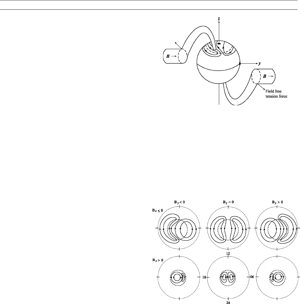
sitely in the two hemispheres. This is illustrated schematically in

Figure M160, which shows a view of the dayside magnetosphere look-

ing from the direction of the Sun shortly after reconnection has taken

place with an IMF having a positive B

component (pointing from left

to right in the figure). The j  B (rubber band) tension force pulls the

newly opened field lines westward (to the left) in the dayside cusp in

the northern hemisphere, and simultaneously eastward (to the right) in

the dayside cusp in the southern hemisphere. The open field lines are

correspondingly carried asymmetrically into the tail lobes, preferen-

tially into the dawn side of the northern lobe, and into the dusk side

of the southern lobe, an effect that tends to twist the tail structure on

the nightside. The corresponding ionospheric flows in the northern

hemisphere are shown in the upper row of diagrams in Figure M161,

for near-zero or negative IMF B

and various IMF B

as indicated.

Again noon is at the top of each diagram and dusk to the left. In this

case the region of open field lines is relatively expanded and the twin

cell Dungey-cycle flows well-developed due to the negative IMF B

while the IMF B

component produces dawn-dusk asymmetries in

the flow with newly opened cusp field lines flowing west for B

posi-

tive (as indicated in Figure M160), and east for B

negative. The

simultaneous east-west flows are opposite in the southern hemisphere.

These variations of the flow in the cusp region (and beyond) produce

corresponding variations in the Hall and Pedersen-FAC current system

that can be sensed both on the ground and above the ionosphere

according to the general principles outlined above. The perturbations

observed at magnetic observatories lying under the cusp (at 75



magnetic latitude near noon) can be used in particular to reconstruct

the large-scale structure of the IMF over long intervals from historic

magnetic records.

Observations indicate that reconnection at the dayside magnetopause

tends to occur preferentially in regions where the magnetospheric and

magnetosheath field adjacent to the magnetopause are antiparallel,

such that the “magnetic gradients” across the boundary are largest.

When the IMF turns from southward to northward, these regions

migrate from low to high latitudes, such that reconnection can then

take place between northward IMF and open field lines in the tail lobes

that were produced by earlier intervals of southward field. Such “lobe

reconnection” does not change the amount of open flux in the tail, but

causes it to circulate within the region of open field lines, as the newly

reconnected field lines flow around the dayside magnetopause and

back into the lobe. The patterns of lobe circulation produced by this

effect are shown in the lower row of diagrams in Figure M161, which

also indicate that the amount of open flux present is usually smaller

under these conditions. Again, these patterns of ionospheric flow are

associated with corresponding patterns of magnetic perturbations

above and below the ionosphere, produced by the corresponding Hall

and Pedersen-FAC currents that are driven.

Figure M160 Schematic of newly opened field lines on the

dayside of the magnetosphere, following low-latitude

reconnection in the presence of an IMF with a positive B

component (directed toward the right). The view is from the

direction of the Sun. Under these conditions the j  B (rubber

band) tension force pulls open field lines westward toward dawn

(left) in the northern hemisphere, and simultaneously eastward

toward dusk (right) in the southern hemisphere, as shown. This

leads to dawn-dusk asymmetries in the dayside ionospheric flow

on open field lines as indicated schematically, which are

oppositely directed in opposite hemispheres.

Figure M161 Sketches of the ionospheric flow in the northern

hemisphere ordered according to the direction of the IMF, in a

format similar to Figure M159. The dashed line shows the

open-closed field line boundary, while the arrowed solid lines

show the plasma streamlines. The upper row show flows for IMF

near zero and negative, while the lower row shows flows

for IMF B

significantly positive. The three columns show flows for

IMF B

negative (left), near zero (center), and positive (right).

Dawn-dusk asymmetries are simultaneously oppositely directed

in the southern hemisphere.

MAGNETOSPHERE OF THE EARTH 661

Magnetospheric substorms

The above sections have discussed the flows and currents that are dri-

ven in the coupled magnetosphere-ionosphere system by the Dungey-

cycle, viewed as a quasisteady process that is strongly modulated by

variations in the strength and direction of the IMF. Observations show,

however, that even when interplanetary conditions are relatively

steady, the driving processes in the key interaction regions at the mag-

netopause and in the geomagnetic tail are not. Reconnection on the

dayside, in particular, often occurs as waves that propagate east-west

over the magnetopause from the dayside toward the tail, which recur

on timescales of 5–10 min. These “flux transfer events” (FTEs) give

rise to pulsed magnetic and plasma signatures at the magnetopause,

and pulsed flow, current, plasma injection, and auroras in the cusp

ionosphere on the dayside. Due to the typically overlapping nature

of the effect of these pulses, however, the overall flow and current

modulations are generally modest.

The pulsed behavior in the tail takes place on longer timescales

of around 1–2 h, however, and produces major perturbations of the

flow and current in the nightside magnetosphere-ionosphere system,

termed magnetospheric substorms (see Storms and substorms). Sub-

storms are initiated by intervals of southward-directed IMF, typically

southward fields of a few nanoteslas lasting for several tens of min-

utes. Such intervals, which happen rather frequently (often several

per day), are sufficient to produce enhanced open flux production at

the dayside magnetopause which in turn enhances the radius and field

strength of the lobes of the tail. The current carried by the plasma sheet

at the center of the tail is also correspondingly intensified, while the

thickness of this current layer is also found to decrease, within the

near-Earth tail, to only a few thousand kilometers. After 30–40 min

of such tail development, termed the “growth phase” of the substorm,

a disruption is observed to occur within the plasma sheet. The origin

and development of the disruption remain controversial, but it involves

the formation within a minute or two of a new reconnection region

within the plasma sheet in the central tail at down-tail distances of

20–30 R

. Reconnection at this site first pinches off the tailward por-

tion of the preexisting plasma sheet, forming a closed-loop plasmoid

field structure, illustrated schematically on the right-hand side of Fig-

ure M158, which is expelled tailward into the solar wind at speeds

in excess 500 km s

–1

. Subsequently, open field lines in the tail lobes

are also reconnected, reducing the amount of open flux in the system.

Earthward of the new reconnection region, new closed field lines col-

lapse toward the Earth, “dipolarizing” the extended tail field lines, and

heating and compressing the plasma sheet plasma. Precipitation from

this hot plasma into the nightside ionosphere produces an expanding

patch of bright active auroras, called the “substorm auroral bulge,”

and also considerably enhances the density of the nightside ionosphere.

Consequently the height-integrated Hall and Pedersen conductivities

in this “bulge” are also strongly enhanced, from 1 mho or less in the

presubstorm nightside ionosphere, to values of 10–100 mho. This

has the effect of suppressing the flow and electric field within the per-

turbed region, but even so intense currents flow within the region, con-

sisting principally of a westward-directed Hall current or “substorm

electrojet.” The total current flow is typically 0.5–1 MA, yielding

magnetic perturbations on the ground underneath the electrojet of sev-

eral hundred nanoteslas. The disturbance field is directed equatorward,

weakening the horizontal component of the planetary dipole field in

both hemispheres. Current continuity is maintained by FACs which

flow from the tail plasma sheet into the ionospheric electrojet at its

eastern end, and return from the ionosphere to the plasma sheet at its

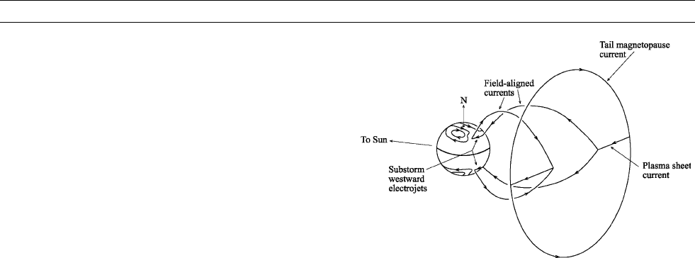
western end, as shown in Figure M162, forming the “substorm current

wedge”. The FACs then close in the cross-tail current on either side of

the dipolarized region, and from thence, over the tail lobe magnetopause

as shown. It can therefore be seen that the current wedge is associated

with a reduction in the cross-tail current within the dipolarized region,

the FACs being associated with the shears in the tail field that occur

in the interface between the dipolarized field within the wedge, and

the (as yet) undipolarized taillike field outside.

As indicated above, substorm tail reconnection and field dipolariza-

tion begin in a localized region near the center of the tail (generally

displaced to the dusk side of midnight), but then spreads in both direc-

tions across the tail. The bright auroral and electrojet current region in

the ionosphere correspondingly starts as a small oval region in the pre-

midnight sector, located typically at 65



magnetic latitude, and then

spreads toward dusk and dawn, as well as poleward as flux continues

to be reconnected and plasma compressed and heated in the nightside

tail. This is called the “expansion phase” of the substorm, and was first

described by Akasofu in 1964. Sometimes the auroral bulge expands

to cover much of the nightside polar ionosphere, though it does not

generally reach to the magnetic pole itself. After 20–30 min the auroral

bulge reaches its maximum size, and the auroral intensity and the cur-

rents then decline, signaling the start of the substorm “recovery phase”

which typically lasts a further 30–40 min. In the tail, “ recovery” is

associated with the down-tail propagation of the new substorm recon-

nection region to large distances from Earth, such that the plasma sheet

re-forms in the near-Earth tail. On the ground underneath the bulge,

where the magnetic effects are dominated by the overhead electrojet

current, the magnetic depression in the horizontal field typically grows

rapidly and impulsively during the expansion phase, and then declines

somewhat more gradually during recovery, giving rise to a signature

which is called a “magnetic bay” in high-latitude magnetic records.

Substorm signatures are also observed in nightside midlatitude mag-

netic fields, but in this case both the ionospheric currents and the FACs

of the current wedge contribute to the form of the overall disturbance.

Several substorm cycles often occur each day, driven by individual

episodes of modest southward field in the IMF, producing magnetic

disturbances in the polar region under the electrojet of 100–1000 nT

which grow and decay over intervals of 1 h. During rarer extended

intervals of strong southward IMF, however, impulsive electrojet

activity is essentially continuously present in the high-latitude nightside

ionosphere, with variable magnetic disturbances on the ground under-

neath peaking at 1000–2000 nT. These high-latitude perturbations

occur simultaneously with worldwide field depressions of typically

50–250 nT which are produced under the same conditions. These

are termed geomagnetic storms and will be discussed in the next section.

The largest high-latitude disturbance observed since systematic records

began in 1957 was of 3000 nT, corresponding to 5% of the planetary

field, this being the largest magnetic effect produced at the Earth’ssurface

Figure M162 Sketch showing the form of the nightside “current

wedge” current system that is excited during the expansion phase

of magnetospheric substorms. A portion of the plasma sheet

current in the center of the tail is diverted along the field lines

north and south toward the Earth, and closes in the ionospheric

substorm westward electrojets. The arrowed vortices drawn

on the sphere representing the Earth’s ionosphere indicate

the concurrent Dungey-cycle flow, similar to Figures M159

and M161.

662 MAGNETOSPHERE OF THE EARTH

due to external currents. At other times, however, the IMF may remain

small and northward-pointing for extended intervals, leading to pro-

longed intervals of “magnetic quiet” on the ground, when only the

variations due to the effects of the Sq-current system are present, driven

by the daily thermal-tidal motions of the upper atmosphere.

Geomagnetic storms

Usually the north-south component of the IMF is a few nanoteslas in

magnitude and fluctuates in sense on timescales of minutes to a few

tens of minutes, as indicated above. This drives variable Dungey-cycle

flows and substorms in the magnetosphere, as discussed in the pre-

vious sections. However, under some rather rare but specific circum-

stances the IMF can become very strong (e.g., several tens of

nanoteslas), and can remain southward-pointing for extended intervals

of several hours. Under these circumstances a geomagnetic storm is

produced at the Earth in which the horizontal (northward) field is

depressed globally over intervals of hours and days, the depression

typically maximizing at a few tens to a few hundreds of nanoteslas.

These effects are masked at high-latitudes, however, by the stronger

and more variable magnetic perturbations associated with magneto-

sphere-ionosphere coupling discussed in the previous section.

For reasons that will be outlined below, the occurrence of magnetic

storms tends to follow the 11-year solar sunspot cycle, as first noted by

Sabine in 1852, but on average there are roughly 10 storms each year

whose midlatitude field depression exceeds 50 nT, and one that

exceeds 250 nT. The largest depression observed since systematic

records began in 1957 was of 600 nT during a storm in March

1989, which occurred near solar maximum. After a variable “initial

phase” to be discussed below, the magnetic depression typically grows

fairly gradually over an interval of several hours (2–12 h), termed the

“main phase,” and then decays even more gradually over the following

several days (1–5 days), termed the “recovery phase.” These effects

result from a prolonged enhancement of the Dungey-cycle flow, which

is produced by the prolonged interval of strong southward IMF. Dur-

ing such intervals the boundary between corotating and Dungey-cycle

flow in the inner equatorial magnetosphere shrinks significantly in

size, such that the outer layers of the preexisting plasmasphere are

stripped off and flow out to the dayside magnetopause. Correspond-

ingly, the hot plasma produced in the tail flows inward to replace it,

significantly enhancing the westward-directed “ring current” produced

by the differential drift of energetic ions and electrons in the inhomo-

geneous quasidipolar planetary magnetic field, as outlined above. The

perturbation field produced by the hot inner plasma is a major contri-

butor to the “main phase” field depression at Earth. However, the pic-

ture is complicated by the fact that the inflowing hot plasma is usually

asymmetric in its distribution around the Earth, leading to partial cur-

rent “rings” that close in the ionosphere via “region 2”-type FACs.

These FACs also contribute to the overall magnetic disturbance, as

do the combined “fringing” fields of the enhanced plasma sheet and

tail currents on the nightside. During the recovery phase, however,

Dungey-cycle convection is reduced, so that these current systems also

decline. Hot “ring current” plasma now marooned within the newly

expanded corotating region slowly decays due to wave-scattering

followed by precipitation into the midlatitude atmosphere, and due

to charge-exchange with neutral atoms of the geocorona. The outer newly

corotating flux tubes also refill with cold plasma from the ionosphere on

timescales of a few days, thus re-forming a more extended plasmasphere.

As indicated at the beginning of this section, the extended intervals

of strong southward IMF which excite geomagnetic storms, are asso-

ciated with specific phenomena in the interplanetary medium which

link storms with processes on the Sun and the solar cycle. Two princi-

pal mechanisms are responsible. In the first, a large loop-like field

structure located in the solar corona suddenly becomes unstable and

is ejected away from the Sun, forming a “coronal mass ejection”

(CME). The ejection speed is sometimes very rapid, exceeding

1000 km s

1

, such that the CME plasma and frozen-in field plow into

the slower solar wind ahead of it. This creates a giant shock wave,

which propagates through the solar system compressing and heating

the ambient solar wind medium ahead of the CME “driver gas”.

Behind the shock the IMF is also compressed to high field strengths.

When such a shock impinges on the Earth, the magnetosphere is

impulsively compressed, such that the horizontal field at the Earth’s

surface is suddenly increased, typically by a few tens of nanoteslas,

corresponding to the effect of the increased Chapman-Ferraro current

at the magnetopause. What happens after this depends on the direction

of the enhanced IMF in the compressed solar wind and CME driver

gas. These fields may have any orientation depending on the indivi-

dual circumstances of the event, and may also fluctuate in direction

during the event. A magnetic storm “main phase” occurs only if the

enhanced IMF points southward during some extended interval after

the shock wave has passed. If this occurs (typically in about one in

six events), the impulsive field enhancement at the Earth’s surface pro-

duced by the shock is called the “storm sudden commencement”

(SSC), while the variable interval between the SSC and the onset of

the main phase (when the upstream IMF happens to turn southward)

is called the “initial phase” of the storm. If such an enduring interval

of southward field does not occur, and with it no “main phase” field

depression, then the shock-related compression event is simply termed

a “sudden impulse”. The connection between these events and

the solar cycle results from the fact that 3 CMEs occur each day near

solar cycle maximum (only a small number of which impinge on

Earth), reducing to one every several days during solar cycle mini-

mum. The connection with solar flares, first noted by Carrington in

1860, results from the fact that flares often occur near the sites in the

solar corona where CMEs have formed.

During the declining phase of the solar cycle, extended intervals of

strong southward IMF can also be produced by another interplanetary

mechanism, which thus can also generate geomagnetic storms. The

Sun typically produces two types of quasisteady solar wind outflow

(as opposed to CMEs), a “slow” variable wind of 300–500 km s

–1

from regions surrounding closed field regions of the solar corona,

and a “fast” steady wind of 800 km s

–1

from open-field “coronal

holes.” During solar maximum, the solar field is typically very disor-

dered, and with it the solar wind outflow. During the declining phase

of the cycle, however, large-scale off-axis coronal holes tend to form,

which migrate slowly toward the poles of the Sun as activity decreases

toward solar minimum. Initially, however, these coronal holes may

extend down to the solar equator, such that during each solar rotation

the Earth experiences a pattern of fast and slow solar wind output that

may persist in form for many solar rotations. The corotating variable

solar wind source regions on the Sun thus give rise to “corotating

interaction regions” (CIRs) in the interplanetary medium, in which fast

plasma outflow from an equatorial coronal hole “runs into” slower

plasma that was emitted earlier into the same direction from a noncor-

onal hole source region on the rotating Sun. This compresses the

plasma and may enhance the frozen-in field by factors of 5–10

above the usual values. As the solar wind velocity subsequently drops,

however, after the passage of the material from the coronal hole, a rar-

efaction region is created in the solar wind, and with it regions of weak

IMF occur. Geomagnetic storms can be excited by the enhanced fields

of the compression phase of CIRs, during intervals in which the solar

wind speed is increasing locally at the Earth, if the enhanced field hap-

pens to point southward for a significant interval. Such storms, however,

are typically not as intense as those generated by CMEs, because the

field directions tend to fluctuate more during these events, as opposed

to the more ordered field structures produced by CMEs. In addition,

these events are not associated with interplanetary shocks, such that

no SSC and “initial phase” occurs prior to the onset of the main phase.

Summary

Overall, it can be seen from this discussion that a variety of interlinked

and rather complex plasma physical processes affect the magnetic field

MAGNETOSPHERE OF THE EARTH 663

observed at the Earth’s surface, and throughout the magnetospheric

region containing the Earth’s magnetic field. The current systems

involved are those concerned with the magnetopause boundary of

the magnetosphere, the hot plasma that flows inside it, and the current

systems that link the magnetosphere and ionosphere and are associated

with the auroras. These produce peak perturbation fields at the Earth’s

surface of typically a few tens, a few hundreds, and a few thousands of

nanoteslas, respectively, varying on a range of timescales from minutes

during substorms to hours and days during worldwide geomagnetic

storms. These current systems are linked to the Sun and solar activity

through the solar wind outflow, which forms the Earth’s magneto-

sphere and conditions its dynamics. The variable output of the Sun

similarly produces effects on a wide range of timescales, from the min-

ute scales associated with interplanetary shocks, up to the 11 year

timescales of the solar activity cycle.

Stanley W.H. Cowley

Bibliography

Cowley, S.W.H., Davies, J.A., Grocott, A., Khan, H., Lester, M.,

McWilliams, K.A., Milan, S.E., Provan, G., Sandholt, P.E., Wild,

J.A., and Yeoman, T.K., 2003. Solar wind-magnetosphere-iono-

sphere interactions in the Earth’s plasma environment. Philosophi-

cal Transactions A, 361:113–126.

Ohtani, S.-I., Fujii, R., Hesse, M., and Lysak, R.L. 2000. Magneto-

spheric Current Systems, Geophysical Monograph 118. Washing-

ton, DC: American Geophysical Union.

Paschmann, G., Haaland, S., and Treumann, R. (eds.), 2002. Auroral

Plasma Physics, Space Science Review, Vol. 103.

Sandholt, P.E., Carlson, H.C., and Egeland, A., 2001. Dayside and

Polar Cap Aurora. Dordrecht: Kluwer Academic Publisher.

Cross-references

Alfvén’s Theorem and the Frozen Flux Approximation

Auroral Oval

Chapman, Sydney (1888–1970)

Ionosphere

Ring Current

Storms and Substorms

MAGNETOSTRATIGRAPHY

Magnetostratigraphy refers to the description, correlation, and dating

of rock sequences by means of magnetic parameters. A rock interval

in which a magnetic parameter has a constant value is called a magne-

tozone. Most commonly, the parameter is the polarity of the Earth’s

magnetic field during acquisition of a primary magnetization that is

contemporaneous with the rock formation. Magnetozones of alternating

polarity yield a magnetic polarity stratigraphy. This form of magnetos-

tratigraphy plays an important role in the construction of geomagnetic

polarity timescales. However, in principle, any rock magnetic parameter

can serve as a magnetostratigraphic indicator.

Although the most widespread and successful use of magnetostrati-

graphy has been in sediments and sedimentary rocks, the method can

be applied to any succession of layered rocks. In igneous rocks and

high-deposition rate sediments, magnetostratigraphy provides fine

details of geomagnetic field behavior. For example, the analysis of

paleomagnetic vectors in radiometrically dated lava flows from Steen’s

Mountain (Oregon, USA) showed details of the behavior of magnetic

field direction and intensity during a Miocene polarity reversal (Prévot

et al., 1985). The study gave an estimated duration of about 4500 years

for the polarity transition. Other estimates range from 3500 to 10000

years. The time intervals (chrons), during which the geomagnetic field

maintains constant normal or reverse polarity, are many times longer

than the transitional interval, and may last hundreds of thousands to

millions of years; they are interspersed with shorter subchrons lasting

only some tens of thousands of years. The reversals apparently occur

at random separations, so that a sequence of reversals defines polarity

chrons and subchrons of very variable lengths. Each polarity reversal

is a global feature, which is very useful for magnetic stratigraphy

because a short sequence of 10–20 reversals forms a distinctive pat-

tern, like a fingerprint, which can be used for geological correlations

on a worldwide basis.

Marine magnetic anomaly sequences

Seafloor spreading since the Middle Jurassic has created sequences of

lineated marine magnetic anomalies in the ocean basins, which have

yielded the most complete and detailed record of geomagnetic polarity

for this time interval. An episode of alternating polarity began about

157 Ma ago in the Late Jurassic and lasted until about 120 Ma ago

in the Early Cretaceous; it gave rise to the M-sequence of marine mag-

netic anomalies. The field apparently rested in a state of normal polar-

ity for the next 37 Ma. A further episode of reversals began 83 Ma ago

in the Late Cretaceous and has lasted throughout the Cenozoic until

the present; it produced a sequence of magnetic anomalies that is

referred to here as the C-sequence. It is possible that the known

C-sequence is incomplete. Short wavelength, low amplitude magnetic

anomalies (so-called “tiny wiggles” or “cryptochrons”) that could cor-

respond to very short-polarity chrons have been observed in the mar-

ine magnetic anomaly record that defines the C-sequence, especially

in the Oligocene and Paleocene. The origin of these magnetic anoma-

lies is uncertain because they can be modeled equally well as short

polarity intervals and intensity fluctuations of the paleomagnetic field

(Cande and LaBrecque, 1974; Cande and Kent, 1992b).

Major magnetic anomalies in each sequence are numbered in order

of increasing age. The corresponding polarity chron is identified with

the prefix “C” in the C-sequence and “CM” in the M-sequence; the

suffix “n” or “r” is appended to designate normal or reverse polarity,

respectively. Thus, the C-sequence of polarity chrons extends from

C1n to C33r, and the M-sequence extends from CM0r to CM29r.

The two anomaly sequences are separated in the oceanic record by

the Cretaceous Quiet Zone (equivalent to C34n) in which lineated

magnetic anomalies are not found. It corresponds to a time interval,

the Cretaceous Normal Polarity Superchron (CNPS), in which the

Earth’s magnetic field did not reverse polarity for more than 37 Ma.

Regions of the oceanic crust older than CM29r form a Jurassic Quiet

Zone, which, like the Cretaceous Quiet Zone, is characterized by the

absence of correlatable magnetic anomalies at the ocean surface.

Deep-tow magnetometer studies have revealed a tentatively correlated

sequence of short wavelength, low amplitude magnetic anomalies

numbered M29-M41 (Sager et al., 1998). These anomalies suggest that

the Jurassic Quiet Zone may result from a high reversal frequency, in

contrast to the origin of the CNPS.

Geomagnetic polarity timescales

The association of radiometric ages with key biostratigraphic stage

boundaries, which have been correlated by magnetostratigraphy to

the marine polarity record, yields a dated geomagnetic polarity time-

scale (GPTS). Several GPTS have been proposed for each reversal

sequence, accompanying refinements in defining the fundamental

polarity record and improvements in confirming, correlating, and dat-

ing the polarity chrons. A comparison of the different GPTS that have

been proposed for the Late Cretaceous and Cenozoic is given by

Opdyke and Channell (1996). A databank of the C-sequence time-

scales has been compiled and stored electronically on-line (Mead,

1996). The optimum GPTS for this time interval is the CK95 timescale

(Cande and Kent, 1995), based upon a reevaluation of the C-sequence

marine magnetic anomalies and the corresponding block models

(Cande and Kent, 1992a).

The M-sequence of marine anomalies is not as well dated as the

C-sequence and it also may still be incomplete. The old end of the

664 MAGNETOSTRATIGRAPHY

M-sequence merges into the Jurassic Quiet Zone, whose origin is less

well understood than its Cretaceous counterpart. A comparison of dif-

ferent GPTS for the M-sequence shows that appreciable discrepancies

still exist. The optimum GPTS for this part of the record is currently

the CENT94 timescale (Channell et al., 1994), which is based on

revised block models for the origin of the marine magnetic anomalies

and covers magnetic polarity chrons CM0 to CM29. Because of their

still uncertain origin, anomalies M29-M41 are not yet accepted as

polarity chrons that can be included in the GPTS.

For each polarity sequence, tie-levels are established by magnetos-

tratigraphic correlation of radiometrically dated biostratigraphic stage

boundaries or other datum-levels to the C- and M-sequence polarity

record. The rest of each timescale is dated by conversion of polarity

boundary locations to numeric ages by interpolation between the tie-

levels. There are several inherent sources of error in this process,

including errors of absolute dating of the stage boundary or other

tie-levels, stratigraphic errors in correlation, etc. Consequently, the

“absolute ages” in a GPTS are known less exactly than the relative

lengths of the polarity chrons.

Magnetic polarity stratigraphy

Methodology

Shallow, unconsolidated sediments from lakes and seas have been

sampled with gravity-driven piston cores, whereas older sediments

from deep ocean basins have been sampled with drilled cores in the

international Ocean Drilling Project (ODP). Indurated sedimentary rocks

can be sampled by ordinary paleomagnetic techniques. Long, continu-

ous, continental outcrops or drillholes are necessary for successful mag-

netostratigraphy. Marine and nonmarine sedimentary rocks that have not

been adversely disturbed by local tectonic conditions have given good

results. Marine rocks can be dated paleontologically, whereas cyclostra-

tigraphy has enabled the dating of some continental deposits.

The sample and data processing methods are the same as in a custom-

ary paleomagnetic study, and strict criteria have been proposed to define

the quality of a magnetostratigraphy (Opdyke and Channell, 1996). It is

possible to measure and partially demagnetize whole cores of sediments

virtually continuously with specially designed pass-through magnet-

ometers. More commonly, the cores are subsampled, either using long,

so-called u-channels or by taking conventional 1 in. paleomagnetic sam-

ples at discrete intervals. Whatever their source, the prepared samples

are treated using standard paleomagnetic methods such as progressive

stepwise demagnetization. In soft wet sediments this treatment is limited

to alternating field demagnetization, which in many cases is quite ade-

quate, as the carrier of remanent magnetization is often primary magne-

tite. Secondary magnetic phases cannot be excluded. In soft marine

sediments obtained from piston cores and ODP they are usually unim-

portant, but in lake sediments the possible presence and effects of

secondary magnetizations carried by minerals such as hematite and grei-

gite must be taken into account. In indurated sedimentary rocks such as

limestones and redbeds, the primary magnetic mineral is usually magne-

tite, but the magnetic mineralogy may be complicated by postdeposi-

tional growth of secondary ferromagnetic minerals. Of these, hematite

is the most common with serious consequences for paleomagnetic inter-

pretation. In this case, progressive partial thermal demagnetization is the

most important laboratory technique for establishing the direction of the

primary magnetization on which the magnetostratigraphy is based.

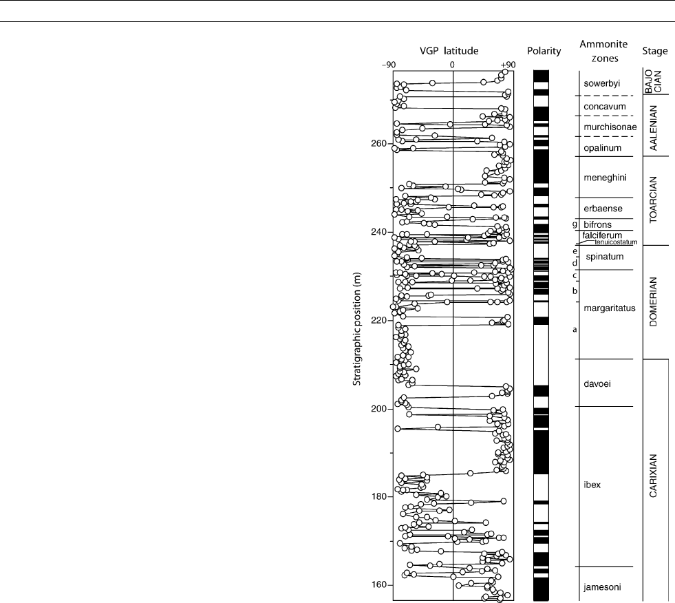
The stable magnetization directions can be used to calculate the lati-

tude of the virtual geomagnetic pole (VGP) at the time of formation of

a sample. The stratigraphic plot of the VGP latitude, or in some cases

the inclination of the magnetization, defines magnetozones of common

polarity (Figure M163). Normal polarity magnetozones are customa-

rily shaded black and reverse polarity zones are left unshaded. Paleon-

tological analyses on samples from the same section based on

ammonites, foraminifera, nannofossils, or other fossil types, define a

biostratigraphy that is tied to the magnetostratigraphy. In this way

the locations of major biostratigraphic stage boundaries are correlated

to the magnetic reversal sequence.

Magnetostratigraphic results often show individual samples with

polarity opposite to adjacent samples. This is often due to misorienta-

tion of the sample, or inadequate magnetic cleaning, but it may be that

some represent very short-lasting polarity chrons.

Magnetostratigraphic verification of the C- and

M-sequences

Magnetic polarity stratigraphy is most successful when a reference

record is available, such as that provided by marine magnetic anoma-

lies since the Late Jurassic. Numerous investigations of magnetic polar-

ity stratigraphy have been carried out in marine limestones and marls

to verify, correlate, and date the history of geomagnetic polarity for

this time interval (Opdyke and Channell, 1996). Studies in continental

exposures of marine limestones have confirmed the main features of

the C- and M-sequences of polarity reversals. Improvements in drilling

technology and the use of pass-through cryogenic magnetometers

have yielded excellent magnetostratigraphies in several ODP studies.

Figure M163 Lower Middle Jurassic magnetic polarity

stratigraphy from the Breggia Gorge, southern Switzerland (after

Horner and Heller, 1983).

MAGNETOSTRATIGRAPHY 665