Jacques I. Mathematics for Economics and Business

Подождите немного. Документ загружается.

Consumers are faced with a choice of how many hours each week to spend working and how

many to devote to leisure. In the same way, a consumer needs to decide how many items of vari-

ous goods to buy and has a preference between the options available. To analyse the behaviour

of consumers quantitatively we associate with each set of options a number, U, called utility,

which indicates the level of satisfaction. Suppose that there are two goods, G1 and G2, and that

the consumer buys x

items of G1 and x

items of G2. The variable U is then a function of x

and x

, which we write as

U = U(x

, x

)

U(3, 7) = 20 and U(4, 5) = 25

for example, then the consumer derives greater satisfaction from buying 4 items of G1 and

5 items of G2 than from buying 3 items of G1 and 7 items of G2.

Utility is a function of two variables, so we can work out two ﬁrst-order partial derivatives,

and

The derivative

gives the rate of change of U with respect to x

and is called the marginal utility of x

. If x

changes by a small amount ∆x

and the other variable is held ﬁxed then the change in U satisﬁes

∆U  ∆x

If x

and x

both change then the net change in U can be found from the small increments

formula

∆U  ∆x

+∆x

∂U

∂x

∂U

∂x

∂U

∂x

∂U

∂x

∂U

∂x

∂U

∂x

Partial Differentiation

360

Example

Given the utility function

U = x

1/4

3/4

determine the value of the marginal utilities

and

when x

= 100 and x

= 200. Hence estimate the change in utility when x

decreases from 100 to 99 and x

increases from 200 to 201.

Solution

U = x

1/4

3/4

∂U

∂x

∂U

∂x

MFE_C05b.qxd 16/12/2005 10:40 Page 360

Note that for the particular utility function

U = x

1/4

3/4

given in the above example, the second-order derivatives

= x

−7/4

3/4

and = x

1/4

−5/4

are both negative. Now ∂

U/∂x

is the partial derivative of marginal utility ∂U/∂x

with respect

to x

. The fact that this is negative means that marginal utility of x

decreases as x

rises. In other

words, as the consumption of good G1 increases, each additional item of G1 bought confers

less utility than the previous item. A similar property holds for G2. This is known as the law of

diminishing marginal utility.

−3

∂

∂x

−3

∂

∂x

5.2 • Partial elasticity and marginal functions

361

then

/4x

−3/4

3/4

and =

/4 x

1/4

−1/4

so when x

= 100 and x

= 200

/4 (100)

−3/4

(200)

3/4

= 0.42

/4 (100)

1/4

(200)

−1/4

= 0.63

Now x

decreases by 1 unit, so

∆x

=−1

and x

increases by 1 unit, so

∆x

= 1

The small increments formula states that

∆U  ∆x

+∆x

The change in utility is therefore

∆U  (0.42)(−1) + (0.63)(1) = 0.21

∂U

∂x

∂U

∂x

∂U

∂x

∂U

∂x

∂U

∂x

∂U

∂x

Advice

You might like to compare this with the law of diminishing marginal productivity discussed

in Section 4.3.2.

MFE_C05b.qxd 16/12/2005 10:40 Page 361

Partial Differentiation

362

Practice Problem

2 An individual’s utility function is given by

U = 1000x

+ 450x

+ 5x

− 2x

− x

where x

is the amount of leisure measured in hours per week and x

is earned income measured in

dollars per week.

Determine the value of the marginal utilities

and

when x

= 138 and x

= 500.

Hence estimate the change in U if the individual works for an extra hour, which increases earned

income by $15 per week.

Does the law of diminishing marginal utility hold for this function?

∂U

∂x

∂U

∂x

It was pointed out in Section 5.1 that functions of two variables could be represented by sur-

faces in three dimensions. This is all very well in theory, but in practice the task of sketching

such a surface by hand is virtually impossible. This difﬁculty has been faced by geographers for

years and the way they circumvent the problem is to produce a two-dimensional contour map.

A contour is a curve joining all points at the same height above sea level. Exactly the same

device can be used for utility functions. Rather than attempt to sketch the surface, we draw an

indifference map. This consists of indifference curves joining points (x

, x

) which give the same

value of utility. Mathematically, an indifference curve is deﬁned by an equation

U(x

, x

) = U

for some ﬁxed value of U

. A typical indifference map is sketched in Figure 5.4.

Points A and B both lie on the lower indifference curve, U

= 20. Point A corresponds to the

case when the consumer buys a

units of G1 and a

units of G2. Likewise, point B corresponds

Figure 5.4

MFE_C05b.qxd 16/12/2005 10:40 Page 362

to the case when the consumer buys b

units of G1 and b

units of G2. Both of these combina-

tions yield the same level of satisfaction and the consumer is indifferent to choosing between

them. In symbols we have

U(a

, a

) = 20 and U(b

, b

) = 20

Points C and D lie on indifference curves that are further away from the origin. The combina-

tions of goods that these points represent yield higher levels of utility and so are ranked above

those of A and B.

Indifference curves are usually downward-sloping. If fewer purchases are made of G1 then

the consumer has to compensate for this by buying more of type G2 to maintain the same level

of satisfaction. Note also from Figure 5.4 that the slope of an indifference curve varies along its

length, taking large negative values close to the vertical axis and becoming almost zero as the

curve approaches the horizontal axis. Again this is to be expected for any function that obeys

the law of diminishing marginal utility. A consumer who currently owns a large number of

items of G2 and relatively few of G1 is likely to value G1 more highly. Consequently, he or she

might be satisﬁed in sacriﬁcing a large number of items of G2 to gain just one or two extra

items of G1. In this region the marginal utility of x

is much greater than that of x

, which

accounts for the steepness of the curve close to the vertical axis. Similarly, as the curve

approaches the horizontal axis, the situation is reversed and the curve ﬂattens off. We quantify

this exchange of goods by introducing the marginal rate of commodity substitution, MRCS.

This is deﬁned to be the increase in x

necessary to maintain a constant value of utility when x

decreases by 1 unit. This is illustrated in Figure 5.5.

Starting at point E, we move 1 unit to the left. The value of MRCS is then the vertical dis-

tance that we need to travel if we are to remain on the indifference curve passing through E.

Now this sort of ‘1 unit change’ deﬁnition is precisely the approach that we took in Section 4.3

when discussing marginal functions. In that section we actually deﬁned the marginal function

to be the derived function and we showed that the ‘1 unit change’ deﬁnition gave a good

approximation to it. If we do the same here then we can deﬁne

MRCS =−

5.2 • Partial elasticity and marginal functions

363

Figure 5.5

MFE_C05b.qxd 16/12/2005 10:40 Page 363

Partial Differentiation

364

Example

Given the utility function

U = x

1/2

ﬁnd a general expression for MRCS in terms of x

and x

Calculate the particular value of MRCS for the indifference curve that passes through (300, 500). Hence

estimate the increase in x

required to maintain the current level of utility when x

decreases by 3 units.

Solution

U = x

1/2

then

/2 x

−1/2

1/2

and =

/2 x

1/2

−1/2

Using the result

MRCS =

∂U/∂x

∂U

∂x

∂U

∂x

The derivative, dx

/dx

, determines the slope of an indifference curve when x

is plotted on the

horizontal axis and x

is plotted on the vertical axis. This is negative, so we deliberately put a

minus sign in front to make MRCS positive. This deﬁnition is useful only if we can ﬁnd the

equation of an indifference curve with x

given explicitly in terms of x

. However, we may only

know the utility function

U(x

, x

)

so that the indifference curve is determined implicitly from an equation

U(x

, x

) = U

This is precisely the situation that we discussed at the end of Section 5.1. The formula for

implicit differentiation gives

=−

Hence

MRCS =− =

marginal rate of commodity substitution is the marginal

utility of x

divided by the marginal utility of x

∂U/∂x

MFE_C05b.qxd 16/12/2005 10:41 Page 364

we see that

MRCS =

= x

−1

At the point (300, 500)

MRCS ==

Now MRCS approximates the increase in x

required to maintain a constant level of utility when x

decreases

by 1 unit. In this example x

decreases by 3 units, so we multiply MRCS by 3. The approximate increase

in x

× 3 = 5

We can check the accuracy of this approximation by evaluating U at the old point (300, 500) and the new

point (297, 505). We get

U(300, 500) = (300)

1/2

(500)

1/2

= 387.30

U(297, 505) = (297)

1/2

(505)

1/2

= 387.28

This shows that, to all intents and purposes, the two points do indeed lie on the same indifference curve.

500

300

/2 x

−1/2

1/2

/2 x

1/2

−1/2

5.2 • Partial elasticity and marginal functions

365

Practice Problem

3 Calculate the value of MRCS for the utility function given in Practice Problem 2 at the point (138, 500).

Hence estimate the increase in earned income required to maintain the current level of utility if leisure

time falls by 2 hours per week.

5.2.3 Production

Production functions were ﬁrst introduced in Section 2.3. We assume that output, Q, depends

on capital, K, and labour, L, so we can write

Q = f(K, L)

Such functions can be analysed in a similar way to utility functions. The partial derivative

∂Q

∂K

MFE_C05b.qxd 16/12/2005 10:41 Page 365

gives the rate of change of output with respect to capital and is called the marginal product of

capital, MP

. If capital changes by a small amount ∆K, with labour held constant, then the

corresponding change in Q is given by

∆Q  ∆K

Similarly,

gives the rate of change of output with respect to labour and is called the marginal product of

labour, MP

. If labour changes by a small amount ∆L, with capital held constant, then the cor-

responding change in Q is given by

∆Q  ∆L

If K and L both change simultaneously, then the net change in Q can be found from the small

increments formula

∆Q  ∆K +∆L

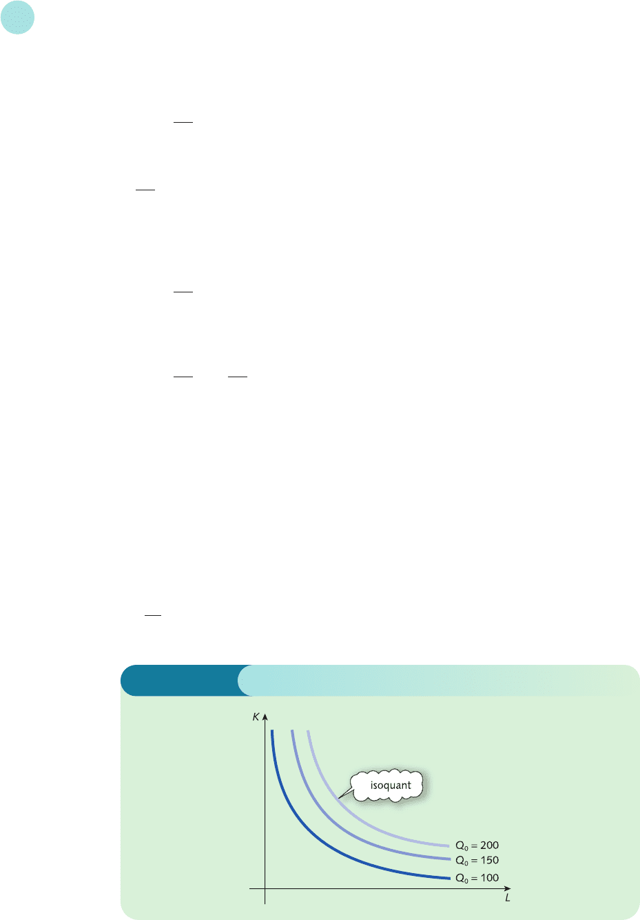
The contours of a production function are called isoquants. In Greek ‘iso’ means ‘equal’, so

the word ‘isoquant’ literally translates as ‘equal quantity’. Points on an isoquant represent all

possible combinations of inputs (K, L) which produce a constant level of output, Q

. A typical

isoquant map is sketched in Figure 5.6. Notice that we have adopted the standard convention

of plotting labour on the horizontal axis and capital on the vertical axis.

The lower curve determines the input pairs needed to output 100 units. Higher levels of

output correspond to isoquants further away from the origin. Again, the general shape of the

curves is to be expected. For example, as capital is reduced it is necessary to increase labour to

compensate and so maintain production levels. Moreover, if capital continues to decrease, the

rate of substitution of labour for capital goes up. We quantify this exchange of inputs by

deﬁning the marginal rate of technical substitution, MRTS, to be

−

∂Q

∂L

∂Q

∂K

∂Q

∂L

∂Q

∂L

∂Q

∂K

Partial Differentiation

366

Figure 5.6

MFE_C05b.qxd 16/12/2005 10:41 Page 366

5.2 • Partial elasticity and marginal functions

367

Practice Problem

4 Given the production function

Q = K

+ 2L

write down expressions for the marginal products

and

Hence show that

(a)

MRTS =

(b) K + L = 2Q

∂Q

∂L

∂Q

∂K

∂Q

∂L

∂Q

∂K

Example

Find an expression for MRTS for the general Cobb–Douglas production function

Q = AK

where A, α and β are positive constants.

Solution

We begin by ﬁnding the marginal products. Partial differentiation of

Q = AK

with respect to K and L gives

=αAK

α−1

and MP

=βAK

β−1

Hence

MRTS == =

βK

αL

βAK

β−1

αAK

α−1

so that MRTS is the positive value of the slope of an isoquant. As in the case of a utility func-

tion, the formula for implicit differentiation shows that

MRTS ==

marginal rate of technical substitution is the marginal product

of labour divided by the marginal product of capital

∂Q/∂L

∂Q/∂K

MFE_C05b.qxd 16/12/2005 10:41 Page 367

Recall that a production function is described as being homogeneous of degree n if, for any

number λ,

f(λK, λL) =λ

f(K, L)

A production function is then said to display decreasing returns to scale, constant returns to

scale or increasing returns to scale, depending on whether n < 1, n = 1 or n > 1, respectively.

One useful result concerning homogeneous functions is known as Euler’s theorem, which

states that

K + L = nf (K, L)

In fact, you have already veriﬁed this in Practice Problem 4(b) for the particular production

function

Q = K

+ 2L

which is easily shown to be homogeneous of degree 2. We have no intention of proving this

theorem, although you are invited to conﬁrm its validity for general Cobb–Douglas production

functions in Practice Problem 10 at the end of this section.

The special case n = 1 is worthy of note because the right-hand side is then simply f(K, L),

which is equal to the output, Q. Euler’s theorem for homogeneous production functions of

degree 1 states that

If each input factor is paid an amount equal to its marginal product then each term on

the left-hand side gives the total bill for that factor. For example, if each unit of labour is

paid MP

then the cost of L units of labour is L(MP

). Provided that the production function

displays constant returns to scale, Euler’s theorem shows that the sum of the factor payments

is equal to the total output.

We conclude this section with an example that shows how the computer package Maple can

be used to handle functions of two variables.

total output

labour times

marginal product

of labour

capital times

marginal product

of capital

∂f

∂L

∂f

∂K

Partial Differentiation

368

Advice

Production functions and the concept of homogeneity were covered in Section 2.3. You

might find it useful to revise this before reading the next paragraph.

Example

Consider the production function

Q = 2K

0.2

0.8

(0 ≤ K ≤ 1000, 0 ≤ L ≤ 1000)

(a) Draw a three-dimensional plot of this function together with its isoquant map.

(b) Use the instruction diff to ﬁnd an expression for MRTS.

MAPLE

MFE_C05b.qxd 16/12/2005 10:41 Page 368

Solution

(a) Let us name this function prod. To do this, we type

>prod:=2*K^0.2*L^0.8;

The instruction for a three-dimensional plot is plot3d. This is used in the same way as ordinary

plot. The only difference is that we must specify the range of both K and L, so we type

>plot3d(prod,K=0..1000,L=0..1000);

If you do this, you get a most uninspiring picture of the surface. Most of the surface is ‘coming straight

towards you’, so you cannot see it properly. Maple does, however, allow you to rotate the surface to get

a better perspective. To do this, click on the surface to make the graphics toolbar appear. This is shown

in Figure 5.7.

5.2 • Partial elasticity and marginal functions

369

Advice

It is well worth playing around with some of the buttons on the toolbar to investigate

some of the useful features of the package. For example, click on the first indicated but-

ton. This creates a cuboid on the screen. To rotate the axes, simply hold the mouse but-

ton down and drag the cursor around. Figure 5.8 (overleaf) shows one such perspective

with the origin at the front. It shows clearly how the output rises with increasing capital

and labour and that this effect is more pronounced with increasing values of L than K.



Figure 5.7

To obtain an isoquant map we need to call up the more sophisticated plotting routines, from which

we select the one called contourplot. You type

>with(plots):

followed by

>contourplot(prod,K=0..1000,L=0..1000);

The response from Maple is the isoquant map shown in Figure 5.9 (overleaf).

(b) Partial differentiation is performed, as usual, via the instruction diff.

Typing

>diff(output,K);

performs the differentiation with respect to K and shows that MP

is given by

0.4L

0.8

MFE_C05b.qxd 16/12/2005 10:41 Page 369