Jacques I. Mathematics for Economics and Business

Подождите немного. Документ загружается.

Partial Differentiation

370

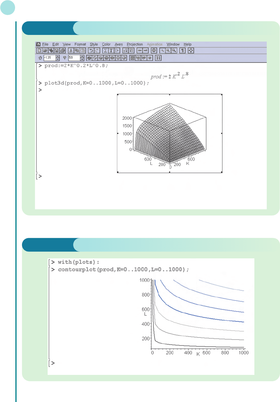
Figure 5.8

Figure 5.9

MFE_C05b.qxd 16/12/2005 10:41 Page 370

5.2 • Partial elasticity and marginal functions

371

Typing

>diff(output,L);

performs the differentiation with respect to L and shows that MP

is given by

The MRTS is found by dividing one by the other. In fact, this can be done in a single line:

>MRTS:=diff(output,L)/diff(output,K);

which gives

MRTS =

1.6K

0.2

Cross-price elasticity of demand The responsiveness of demand for one good to a change

in the price of another: (percentage change in quantity) ÷ (percentage change in the price of

the alternative good).

Euler’s theorem If each input is paid the value of its marginal product, the total costs of

these inputs is equal to total output, provided there are constant returns to scale.

Income elasticity of demand The responsiveness of demand for one good to a change in

income: (percentage change in quantity) ÷ (percentage change in income).

Indifference curves A curve indicating all combinations of two goods which give the same

level of utility.

Indifference map A diagram showing the graphs of a set of indifference curves. The further

the curve is from the origin, the greater the level of utility.

Isoquant A curve indicating all combinations of two factors which give the same level of

output.

Law of diminishing marginal utility The law which states that the increase in utility due

to the consumption of an additional good will eventually decline: ∂

U/∂x

< 0 for sufﬁciently

large x

Marginal product of capital The additional output produced by a 1 unit increase in

capital: MP

=∂Q/∂K.

Marginal product of labour The additional output produced by a 1 unit increase in labour:

=∂Q/∂L.

Marginal rate of commodity substitution The amount by which one input needs to

increase to maintain a constant value of utility when the other input decreases by 1 unit:

MRTS =∂U/∂x

÷∂U/∂x

Marginal rate of technical substitution The amount by which capital needs to rise to

maintain a constant level of output when labour decreases by 1 unit: MRTS = MP

/MP

Marginal utility The extra satisfaction gained by consuming 1 extra unit of a good: ∂U/∂x

Price elasticity of demand The responsiveness of demand for one good to a change in its

own price: − (percentage change in quantity) ÷ (percentage change in the price).

Utility The satisfaction gained from the consumption of a good.

Key Terms

MFE_C05b.qxd 16/12/2005 10:41 Page 371

Partial Differentiation

372

Practice Problems

5 Given the demand function

Q = 200 − 2P − P

+ 0.1Y

where P = 10, P

= 15 and Y = 100, find

(a) the price elasticity of demand

(b) the cross-price elasticity of demand

Estimate the percentage change in demand if P

rises by 3%. Is the alternative good substitutable or

complementary?

6 Given the demand function

Q =

where P

= 10, Y = 2 and P = 4, find the income elasticity of demand. If P

and P are fixed, estimate

the percentage change in Y needed to raise Q by 2%.

7 Given the utility function

U = x

1/2

1/3

determine the value of the marginal utilities

and

at the point (25, 8). Hence

(a) estimate the change in utility when x

and x

both increase by 1 unit

(b) find the marginal rate of commodity substitution at this point

8 Evaluate MP

and MP

for the production function

Q = 2LK + L

given that the current levels of K and L are 7 and 4, respectively. Hence

(a) write down the value of MRTS

(b) estimate the increase in capital needed to maintain the current level of output given a 1 unit

decrease in labour

9 If Q = 2K

+ 3L

K show that K(MP

) + L(MP

) = 3Q.

10 Verify Euler’s theorem for the Cobb–Douglas production function

Q = AK

[Hint: this function was shown to be homogeneous of degree α+βin Section 2.3.]

11 If a firm’s production function is given by

Q = 5L + 7K

sketch the isoquant corresponding an output level, Q = 700. Use your graph to find the value of

MRTS and confirm this using partial differentiation.

∂U

∂x

∂U

∂x

MFE_C05b.qxd 16/12/2005 10:41 Page 372

12 (Maple) Consider the production function

Q = L(5 K + L) (0 ≤ K ≤ 3, 0 ≤ L ≤ 5)

(a) Draw a three-dimensional plot of this function. Rotate the axes to give a clear view of the sur-

face. Draw the corresponding isoquant map.

(b) Find an expression for MRTS.

13 (Maple) Consider the production function

Q = (0.3K

−3

+ 0.7L

−3

)

−1/3

(1 ≤ K ≤ 10, 1 ≤ L ≤ 10)

(a) Draw a three-dimensional plot of this function. Rotate the axes to give a clear view of the surface.

(b) Draw the corresponding isoquant map. Deduce that the marginal rate of technical substitution

diminishes with increasing L.

(d) Find the slope of the isoquant Q = 4 at the point L = 8.

5.2 • Partial elasticity and marginal functions

373

MFE_C05b.qxd 16/12/2005 10:41 Page 373

section 5.3

Comparative statics

The simplest macroeconomic model, discussed in Section 1.6, assumes that there are two sec-

tors, households and ﬁrms, and that household consumption, C, is modelled by a linear rela-

tionship of the form

C = aY + b (1)

In this equation Y denotes national income and a and b are parameters. The parameter a is the

marginal propensity to consume and lies in the range 0 < a < 1. The parameter b is the

autonomous consumption and satisﬁes b > 0. In equilibrium

Y = C + I (2)

Objectives

At the end of this section you should be able to:

 Use structural equations to derive the reduced form of macroeconomic models.

 Calculate national income multipliers.

 Use multipliers to give a qualitative description of economic models.

 Use multipliers to give a quantitative description of economic models.

 Calculate multipliers for the linear one-commodity market model.

Advice

The content of this section is quite difficult since it depends on ideas covered earlier in this

book. You might find it helpful to read quickly through Section 1.6 now before tackling

the new material.

MFE_C05c.qxd 16/12/2005 10:41 Page 374

5.3 • Comparative statics

375

where I denotes investment, which is assumed to be given by

I = I* (3)

for some constant I*. Equations (1), (2) and (3) describe the structure of the model and as such

are called structural equations. Substituting equations (1) and (3) into equation (2) gives

Y = aY + b + I*

Y − aY = b + I* (subtract aY from both sides)

(1 − a)Y = b + I* (take out a common factor of Y )

Y = (divide both sides by 1 − a)

This is known as the reduced form because it compresses the model into a single equation

in which the endogenous variable, Y, is expressed in terms of the exogenous variable, I*, and

parameters, a and b. The process of analysing the equilibrium level of income in this way is

referred to as statics because it assumes that the equilibrium state is attained instantaneously.

The branch of mathematical economics which investigates time dependence is known as

dynamics and is considered in Chapter 9.

We should like to do rather more than just to calculate the equilibrium values here. In par-

ticular, we are interested in the effect on the endogenous variables in a model brought about

by changes in the exogenous variables and parameters. This is known as comparative statics,

since we seek to compare the effects obtained by varying each variable and parameter in turn.

The actual mechanism for change will be ignored and it will be assumed that the system returns

to equilibrium instantaneously. The equation

Y =

shows that Y is a function of three variables, a, b and I*, so we can write down three partial

derivatives

The only hard one to work out is the ﬁrst, and this is found using the chain rule by writing

Y = (b + I*)(1 − a)

−1

which gives

= (b + I*)(−1)(1 − a)

−2

(−1) =

To interpret this derivative let us suppose that the marginal propensity to consume, a, changes

by ∆a with b and I* held constant. The corresponding change in Y is given by

∆Y =∆a

Strictly speaking, the ‘=’ sign should really be ‘’. However, as we have seen in the previous two

sections, provided that ∆a is small the approximation is reasonably accurate. In any case we

could argue that the model itself is only a ﬁrst approximation to what is really happening in the

economy and so any further small inaccuracies that are introduced are unlikely to have any

signiﬁcant effect on our conclusions. The above equation shows that the change in national

income is found by multiplying the change in the marginal propensity to consume by the par-

tial derivative ∂Y/∂a. For this reason the partial derivative is called the marginal propensity to

consume multiplier for Y. In the same way, ∂Y/∂b and ∂Y/∂I* are called the autonomous con-

sumption multiplier and the investment multiplier, respectively.

∂Y

∂a

b + I*

(1 − a)

∂Y

∂a

∂Y

∂I*

∂Y

∂b

∂Y

∂a

b + I*

1 − a

b + I*

1 − a

MFE_C05c.qxd 16/12/2005 10:41 Page 375

Partial Differentiation

376

Multipliers enable us to explain the behaviour of the model both qualitatively and quantita-

tively. The qualitative behaviour can be described simply by inspecting the multipliers as they

stand, before any numerical values are assigned to the variables and parameters. It is usually

possible to state whether the multipliers are positive or negative and hence whether an increase

in an exogenous variable or parameter leads to an increase or decrease in the corresponding

endogenous variable. In the present model it is apparent that the marginal propensity to con-

sume multiplier for Y is positive because it is known that b and I* are both positive, and the

denominator (1 − a)

is clearly positive. Therefore, national income rises whenever a rises.

Once the exogenous variables and parameters have been assigned speciﬁc numerical values,

the behaviour of the model can be explained quantitatively. For example, if b = 10, I* = 30 and

a = 0.5 then the marginal propensity to consume multiplier is

==160

This means that when the marginal propensity to consume rises by, say, 0.02 units the change

in national income is

160 × 0.02 = 3.2

Of course, if a, b and I* change by amounts ∆a, ∆b and ∆I* simultaneously then the small

increments formula shows that the change in Y can be found from

∆Y =∆a +∆b +∆I*

∂Y

∂I*

∂Y

∂b

∂Y

∂a

10 + 30

(1 − 0.5)

b + I*

(1 − a)

Example

Use the equation

Y =

to ﬁnd the investment multiplier.

Deduce that an increase in investment always leads to an increase in national income.

Calculate the change in national income when investment rises by 4 units and the marginal propensity

to consume is 0.6.

Solution

Writing

Y =+

we see that

which is positive because a < 1. Therefore national income rises whenever I* rises.

When a = 0.6 the investment multiplier is

===2.5

so that when investment rises by 4 units the change in national income is

2.5 × 4 = 10

0.4

1 − 0.6

1 − a

∂Y

∂I*

1 − a

b + I*

1 − a

MFE_C05c.qxd 16/12/2005 10:41 Page 376

5.3 • Comparative statics

377

The following example is more difﬁcult because it involves three sectors: households, ﬁrms

and government. However, the basic strategy for analysing the model is the same. We ﬁrst

obtain the reduced form, which is differentiated to determine the relevant multipliers.

These can then be used to discuss the behaviour of national income both qualitatively and

quantitatively.

Practice Problem

1 By substituting

Y =

into

C = aY + b

write down the reduced equation for C in terms of a, b and I*. Hence show that the investment mul-

tiplier for C is

Deduce that an increase in investment always leads to an increase in consumption. Calculate the

change in consumption when investment rises by 2 units if the marginal propensity to consume is

/2.

1 − a

b + I*

1 − a

Example

Consider the three-sector model

Y = C + I + G (1)

C = aY

+ b (0 < a < 1, b > 0) (2)

= Y − T (3)

T = tY + T* (0 < t < 1, T* > 0) (4)

I = I*(I* > 0) (5)

G = G*(G* > 0) (6)

where G denotes government expenditure and T denotes taxation.

(a) Show that

Y =

(b) Write down the government expenditure multiplier and autonomous taxation multiplier. Deduce the

direction of change in Y due to increases in G* and T*.

taxation, ∆T *, so that

∆G* =∆T*

show that national income rises by an amount that is less than the rise in expenditure.

(d) If a = 0.7, b = 50, T* = 200, t = 0.2, I * = 100 and G* = 300, calculate the equilibrium level of national

income, Y, and the change in Y due to a 10 unit increase in government expenditure.

−aT * + b + I* + G*

1 − a + at



MFE_C05c.qxd 16/12/2005 10:41 Page 377

Partial Differentiation

378

Solution

(a) We need to ‘solve’ equations (1)–(6) for Y. An obvious ﬁrst move is to substitute equations (2), (5) and

(6) into equation (1) to get

Y = aY

+ b + I* + G* (7)

Now from equations (3) and (4)

= Y − T

= Y − (tY + T*)

= Y − tY − T*

so this can be put into equation (7) to get

Y = a(Y − tY − T *) + b + I* + G*

= aY − atY − aT* + b + I* + G*

Collecting terms in Y on the left-hand side gives

(1 − a + at)Y =−aT * + b + I* + G*

which produces the desired equation

Y =

(b) The government expenditure multiplier is

and the autonomous taxation multiplier is

We are given that a < 1, so 1 − a > 0. Also, we know that a and t are both positive, so their product, at,

must be positive. The expression (1 − a) + at is therefore positive, being the sum of two positive terms.

The government expenditure multiplier is therefore positive, which shows that any increase in G* leads

to an increase in Y. The autonomous taxation multiplier is negative because its numerator is negative

and its denominator is positive. This shows that any increase in T* leads to a decrease in Y.

∆G* =∆T*

From the small increments formula

∆Y =∆G* +∆T*

we deduce that

∆Y =+∆G* =+∆G* =∆G*

The multiplier

1 − a

1 − a + at

1 − a

1 − a + at

−a

1 − a + at

∂Y

∂T*

∂Y

∂G*

∂Y

∂T*

∂Y

∂G*

−a

1 − a + at

∂Y

∂T*

1 − a + at

∂Y

∂G*

−aT * + b + I* + G*

1 − a + at

MFE_C05c.qxd 16/12/2005 10:41 Page 378

5.3 • Comparative statics

379

is called the balanced budget multiplier and is positive because the numerator and denominator are

both positive. An increase in government expenditure leads to an increase in national income. How-

ever, the denominator is greater than the numerator by an amount at, so that

< 1

and ∆Y <∆G*, showing that the rise in national income is less than the rise in expenditure.

(d) To solve this part of the problem we simply substitute the numerical values a = 0.7, b = 50, T* = 200,

t = 0.2, I* = 100 and G* = 300 into the results of parts (a) and (b). From part (a)

Y == =704.5

From part (b) the government expenditure multiplier is

==2.27

and we are given that ∆G* = 10, so the change in national income is

2.27 × 10 = 22.7

0.44

1 − a + at

−0.7(200) + 50 + 100 + 300

1 − 0.7 + 0.7(0.2)

−aT * + b + I* + G*

1 − a + at

1 − a

1 − a + at

Practice Problem

2 Consider the four-sector model

Y = C + I + G + X − M

C = aY + b (0 < a < 1, b > 0)

I = I*(I* > 0)

G = G*(G* > 0)

X = X *(X* > 0)

M = mY + M* (0 < m < 1, M* > 0)

where X and M denote exports and imports respectively and m is the marginal propensity to import.



MFE_C05c.qxd 16/12/2005 10:41 Page 379