Литвин Ф.Л. Развитие технологии и теории зубчатых передач

Подождите немного. Документ загружается.

NASA RP–1406 33

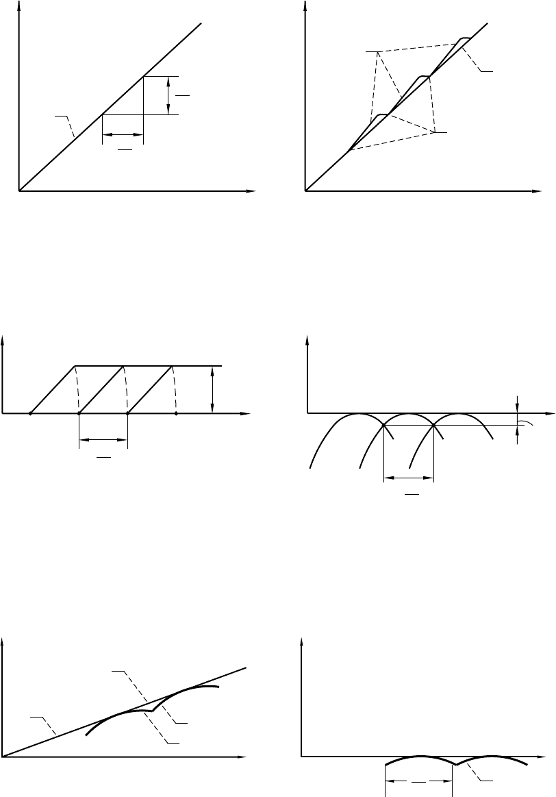
Figure 1.14.1.—Transmission functions of ideal and misaligned gear drives. (a) Ideal.

(b) Misaligned.

(a)

(b)

Points of

transfer

Figure 1.14.2.—Function of transmission errors for gears. (a) Existing geometry. (b) Modified geometry.

2max

(a) (b)

Figure 1.14.3.—Transmission function and function of transmission errors for misaligned gear drive.

(a) 1, ideal transmission function; 2, transmission function for gears with modified geometry. (b) 3,

predesigned parabolic function of transmission errors.

(b)

(a)

)

34 NASA RP–1406

Interaction of Parabolic and Linear Functions of Transmission Errors

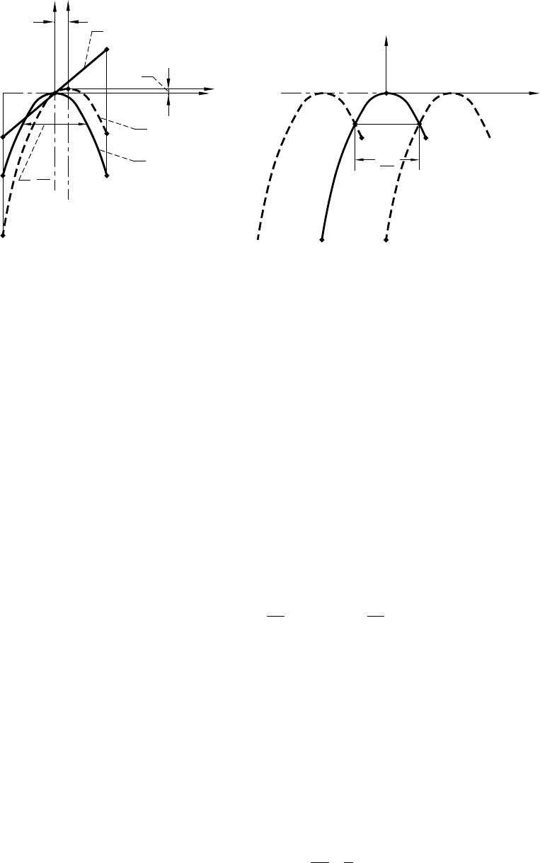
Figure 1.14.4(a) shows the interaction of two functions: (1) the linear function ∆

(1)

= b

caused by gear

misalignment and (2) the predesigned parabolic function ∆

(2)

= –a

provided by the modification of the

contacting gear tooth surfaces. Our goal is to prove that the linear function ∆

(1)

(

) will be absorbed because

of the existence of the parabolic function ∆

(2)

= –a

. To prove it, we consider the resulting function of

transmission errors to be

∆∆ ∆φφ φ φ φ φ φ φ

111

1143() () () (..)

() ( )

=+=−ba

The proof is based on the consideration that equation (1.14.3) represents in a new coordinate system with axes

(∆

) (fig. 1.14.4(a)) the parabolic function

∆ψ ψ

1144 =−a (. .)

The axes of coordinate systems (∆

) and (∆

) are parallel but their origins are different. The

coordinate transformation between the coordinate systems above is represented by

∆∆ψφ ψφ

1145=− =−

,(..)

Equations (1.14.3) and (1.14.5), considered simultaneously, yield equation (1.14.4). Thus, the linear function

∆

(1)

(

) is indeed absorbed because of its interaction with the predesigned parabolic function ∆

(2)

(

). This

statement is in agreement with the transformation of equations of second-order curves discussed in the

mathematics literature (Korn and Korn, 1968).

The difference between the predesigned parabolic function ∆

(2)

(

) and the resulting parabolic function

∆

(

) is the location of points (A*,B*) in comparison with (A,B). Figure 1.14.4(a) shows that the symmetrical

location of (A,B) is turned into the asymmetrical location of (A*,B*). However, the interaction of several

functions ∆

(

), determined for several neighboring tooth surfaces, provides a symmetrical parabolic

function of transmission errors ∆

(

) as shown in figure 1.14.4(b). (The neighboring tooth surfaces enter into

mesh in sequence.) The symmetrical shape of function ∆

(

) determined for several cycles of meshing can

be achieved if the parabolic function ∆

(2)

(

) is predesigned in the area (fig. 1.14.4(a))

φφ

1146() () (. .)BA

−≥+

The requirement (1.14.6), if observed, provides a continuous symmetrical function ∆

(

) for the range of

the meshing cycle

= 2π/N

Figure 1.14.4.—Interaction of parabolic and linear functions. (a) Linear and parabolic functions of

transmission errors. (b) Resulting function of transmission errors.

(b)

(a)

(2)

= bf

= – ac

(1)

= – af

NASA RP–1406 35

Appendix A

Parallel Transfer of Sliding Vectors

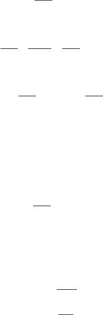
A sliding vector a is determined by its magnitude |a| and the line of its action A

-A (fig. A.1), along which

it can be moved. Examples of a sliding vector are forces and angular velocities. In the last case, the line of action

-A is the axis of rotation.

The parallel transfer of a sliding vector means that a can be substituted by a* = a and a vector moment

mRa=× (.)A1

where R is a position vector drawn from point O of the line of action of a* to any point of the line of action of

a. It is easy to prove that the vector moment m, for instance, can be expressed as (fig. A.1)

ma=×OA

2(.)A

Taking into account that

Ra=+ =+OA A A OA

00 0

3*(.)

where

is a scalar factor, we obtain

mRa= a a a=× +

()

×= ×OA OA

(.)A

Figure A.2 is an example of a sliding vector as the angular velocity of rotation

about the axis A

-A. The

axis of rotation does not pass through the origin O of the considered coordinate system S(x,y,z). The velocity

of point M in rotation about A

-A can be determined using the following procedure:

Step 1: We substitute vector

that passes through A

by a parallel and equal vector

* that passes through O

and the vector moment

m =×OA

ωω

(.)A

where m is a free vector that represents the velocity of translation.

Step 2: The motion of point M is represented now in two components: (1) as translation with the velocity m and

(2) as rotation about OO* with the angular velocity

* =

Step 3: The velocity of rotation of point M about the axis

OO*

is determined as

rot

=×

ωω

*(.)OM A6

36 NASA RP–1406

Figure A.1.—Representation of sliding vector.

Figure A.2.—Substitution of sliding vector.

NASA RP–1406 37

Step 4: The whole velocity of point M is determined as

vrR=×

()

+×

()

=×−OA OM

ωωωωωω

() (.)A

where r =

and R =

Step 5: It is easy to verify that equation (A.7) may be interpreted as

v =×

ωωρρ

(.)A8

where

= r – R =

represents the position vector drawn from point A

of the axis of rotation A

-A to point

M. A position vector

* may be drawn to M from any point on the line of action A

-A. For instance, we may

consider that

* =

AM*

(not shown in the figure) and represent v as

v =×

ωω

A*M (.)A9

Taking into account that

AM AA AM AM** (.)

=+=+

00 0 0

a A

we obtain

va=× =× +

()

=×

ωωωωρρωωρρ

A* M

*(.)A11

since

ωω

*(.)a =0 A12

because of the collinearity of vectors.

Equations (A.7) and (A.8) enable one to determine the velocity of point M by two alternate approaches.

Henceforth, we will use the approach that is based on the substitution of sliding vector

with an equal vector

* and the vector of translation m.

Problem A.1. Represent analytically vector velocity v of point M by considering as given (fig. A.2)

ωω

[]

ωγγ

000

sin cos , – ,

OA E OM x y zR

Solution.

vrR

ijk

ωω

()

−













– sin cos

sin cos

( )cos

–( )sin

(. )

ff f

xE y z

013

ωω ωγγ

γγ

38 NASA RP–1406

Appendix B

Screw Axis of Motion: Axodes

B.1 Screw Motion

Generally, the motion of a rigid body may be represented as a screw motion—rotation about and translation

along an axis called the axis of screw motion.

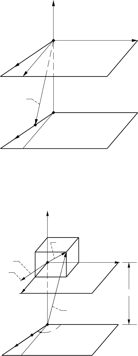
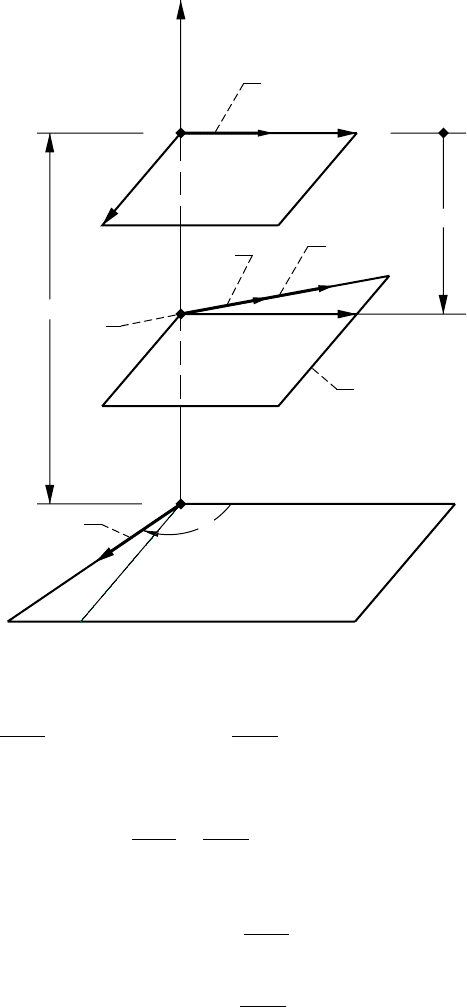
Figure B.1.1 shows that gears 1 and 2 perform rotation about crossed axes with angular velocities

(1)

and

(2)

. The instantaneous relative motion of gear 1 may be represented as a screw motion with parameter p about

the S-S axis that lies in plane Π that is parallel to vectors

(1)

and

(2)

. To determine the location of plane Π

and the screw parameter p, we use the following procedure:

Step 1: Substitute vectors

(1)

and –

(2)

with equal vectors that lie in plane Π and with respective vector

moments

OO OO

() () () ()

, – ( . . )

112 2

11=

()

×=

()

ωωωω

The subscript f indicates that vectors in equations (B.1.1) are represented in coordinate system S

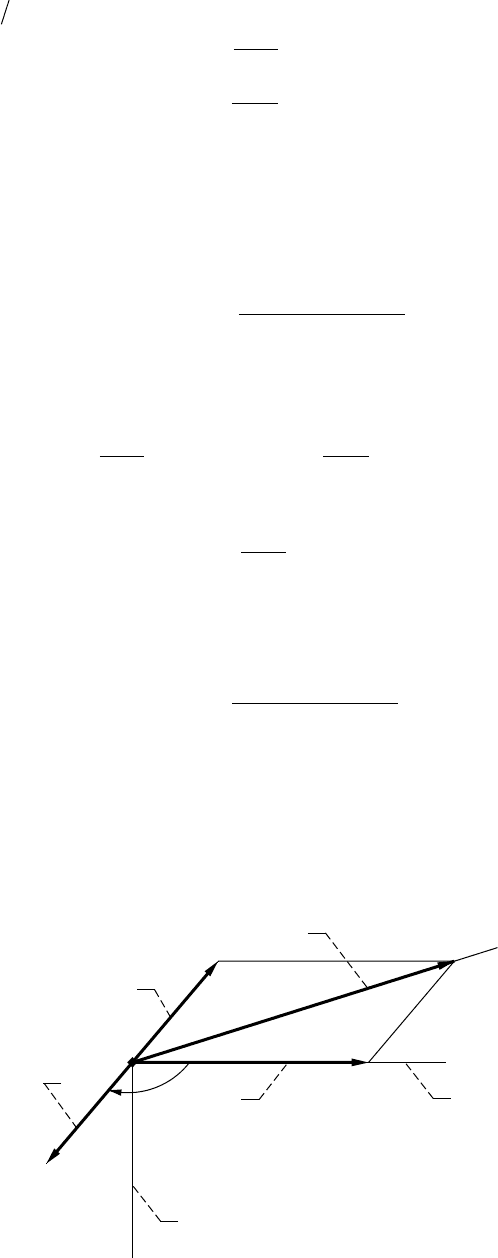
Step 2: The angular velocity in relative motion

(12)

is represented as (fig. B.1.2)

ωωωωωωωωωωωω

ff f

( ) () () () () ()

– sin cos ( . . )

12 1 2 2 1 2

12=+

()

=− + −

()

γγ

jkB

The resulting vector moment is

mmm

fff

OO OO

( ) () () () ()

(..)

12 1 2 1 2

13=+= ×

()

+×−

ωωωω

Step 3: Vector moment m

(12)

is a function of

= X

.. Our next goal is to make m

(12)

collinear to

(12)

and this requirement can be represented by

OO OO p

()

×−

()

×=

ωωωωωω

() () ( )

(..)

1212

Drawings of figure B.1.1 show that

OO O O OO

=+ (..)B15

Equations (B.1.4) and (B.1.5) yield

OO OO p

()

×−

()

×=

ωωωωωω

() () ()

(..)

12 2 12

Step 4: The determination of

= X

is based on the following transformation of equation (B.1.6):

NASA RP–1406 39

ωωωωωωωωωωωω

fff

OO OO p

() () () () () ()

(..)

12 12 12 2 12 12

017×

()













−×

()













=×

()

Equation (B.1.7) yields

ωωωωωω

OO O O

() () ()

(..)

12 2

018

()

−

()

⋅

()

since

−⋅

()













ωωωω

() ()

(..)

12 12

019B

−⋅

()













ωωωω

() ( )

(.. )

212

0110

The scalar products of vectors in equations (B.1.9) and (B.1.10) are equal to zero because of the

perpendicularity of cofactor vectors.

Vectors of equation (B.1.8) are represented as (fig. B.1.1)

ωω

( ) () () ()

()

sin cos

sin cos ( . . )

12 2 1 2

21 21

1111

=− + −

()

=− +−

()

[]

ωωω

γγ

jk B

Figure B.1.1.—Screw axis of rotation.

(2)

(12)

(1)

40 NASA RP–1406

where

ωω

() ()

OO X

fff

= i (.. )B112

OO E

=− i (.. )B113

ωω

() ()

cos ( . . )

114=+

()

sin

γγ

jk B

The orientation of

(12)

and axis S-S of screw motion is illustrated by the drawings of figure B.1.2.

Equations (B.1.8) and (B.1.11) to (B.1.14) yield

−

()

−+

21 21

115

cos

(.. )

Step 5: The determination of the screw parameter p is based on the following transformation of

equation (B.1.7):

ωωωωωωωωωω

OO OO p

() () () () ()

(.. )

12 12 12 2 12

116⋅

()













−⋅

()













()

Here

ωωωω

() ()

(.. )

12 12

0117⋅

()













= B

because of the collinearity of two cofactor vectors in the triple product.

Equations (B.1.16) and (B.1.17) yield the following expression for p:

118

sin

cos

(.. )

1–2

For the case when the rotation of gear 2 is opposite to that shown in figure B.1.1, it is necessary to make m

negative in equations (B.1.15) and (B.1.18). A negative value of X

in equation (B.1.15) indicates that plane Π

intersects the negative axis x

. A negative value of p indicates that vector p

(12)

is opposite the direction shown

in figure B.1.1.

Figure B.1.2.—Relative angular velocity.

(1)

(2)

– v

(2)

(12)

Parallel

to z

Parallel

to x

NASA RP–1406 41

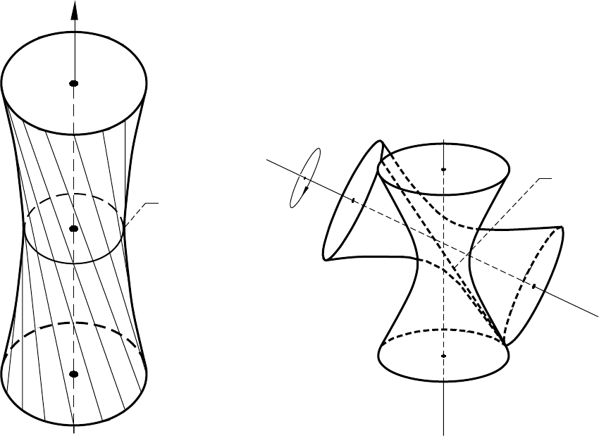
B.2 Axodes

For the case of rotation between crossed axes with a constant gear ratio, the axodes are two hyperboloids of

revolution. The axode of gear i (i = 1,2) is formed as a family of instantaneous axes of screw motion that is

generated in coordinate system S

when gear i is rotated about its axis. An axode as a hyperboloid of revolution

is shown in figure B.2.1. Two mating hyperboloids (fig. B.2.2) contact each other along a straight line that is

the axis of screw motion. The relative motion of hyperboloids is rolling with sliding (about and along the axis

of screw motion).

In the real design of gears with crossed axes, pitch surfaces instead of axodes are applied. In cases of worm-

gear drives and hypoid gear drives, the pitch surfaces are two cylinders and two cones, respectively (Litvin,

1968, 1989). The point of tangency of pitch surfaces is one of the points of tangency of gear tooth surfaces.

Figure B.2.2.—Mating hyperboloids.

Axis of

screw

motion

Figure B.2.1.—Hyperboloid of revolution.

Throat of

hyperboloid

42 NASA RP–1406

Appendix C

Application of Pluecker’s Coordinates and Linear

Complex in Theory of Gearing

C.1 Introduction

This appendix covers the basic concepts of Pluecker’s coordinates, Pluecker’s equation for a straight line,

and Pluecker’s linear complex (Pluecker, 1865). It is shown that applying the linear complex enables one to

illustrate the vector field in the screw motion and to interpret geometrically the equation of meshing and the two-

parameter enveloping process.

Many scientists considered Pluecker’s ideas to have been a significant contribution to the theory of line

geometry (e.g., the work by Klein 1939; Bottema and Roth 1979; and Hunt, 1978).

The concepts of Pluecker’s coordinates and linear complex were applied to the theory of gearing by Brandner

(1983, 1988) and Grill (1993) and Häussler et al. (1996). This section is limited to Pluecker’s representation

of a directed line, his linear complex, and the application of these to the theory of gearing.

C.2 Pluecker’s Presentation of Directed Line

A straight line in a space is determined by a given position vector r

of a point M

of the line and by a directed

vector a that is parallel to the straight line (fig. C.2.1). The parametric representation of a directed straight line

r r r a =+ =+ ≠ ∈

oo o

MM Aλλ λ( ), ( . . )021C

The straight line is directed in accordance with the sign of the scalar factor λ.

If it is assumed that a passes through M

, the moment of the directed straight line with respect to origin O is

determined as

mra

=× (..)C22

It is easy to verify that

ra r a ar am×=

()

××

+==

(..)C23

ma raa

⋅= ×

()

⋅=024(..)C

Equations

mra=rama

oaa

= ×× ⋅=,(..)025C

are satisfied for any current point of the straight line. These equations determine a straight line and called

Pluecker’s equations of a straight line. Therefore, six coordinates ((a

), (m

)) are called Pluecker’s

coordinates. Only four of these coordinates are independent since m

· a = 0 and have a common scalar factor.

We may, for instance, consider a

= a/|a|, and m

* = r × a

instead of a and m