Masujima M. Applied Mathematical Methods in Theoretical Physics

Подождите немного. Документ загружается.

7.2 Homogeneous Wiener–Hopf Integral Equation of the Second Kind 237

based on the requirement that

inc

(



x , t) → 0ast →−∞,

but it grows exponentially in time, i.e.,

inc

= e



p·



x−ωt)

Im ω>0,

is known as turning on the perturbation adiabatically.

7.2

Homogeneous Wiener–Hopf Integral Equation of the Second Kind

The Wiener–Hopf integral equations are characterized by translation kernels,

K(x, y) = K(x −y), and the integral is on the semi-inﬁnite range,0< x, y < ∞.

We list the Wiener–Hopf integral equations of several types.

Wiener–Hopf integral equation of the ﬁrst kind:

F(x) =



+∞

K(x − y)φ(y)dy,0≤ x < ∞.

Homogeneous Wiener–Hopf integral equation of the second kind:

φ(x) = λ



+∞

K(x − y)φ(y)dy,0≤ x < ∞.

Inhomogeneous Wiener–Hopf integral equation of the second kind:

φ(x) = f (x) + λ



+∞

K(x − y)φ(y)dy,0≤ x < ∞.

Let us begin with the homogeneous Wiener–Hopf integral equation of the second kind:

φ(x) = λ



+∞

K(x − y)φ(y)dy,0≤ x < ∞. (7.2.1)

Here, the translation kernel K(x −y) is deﬁned for its argument both positive and

negative. Suppose that

K(x) →



−bx

as x →+∞,

as x →−∞,

a, b > 0, (7.2.2)

so that the Fourier transform of K(x), deﬁned by

K(k) =



+∞

−∞

dxe

−ikx

K(x), (7.2.3)

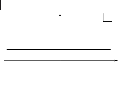
238 7 Wiener–Hopf Method and Wiener–Hopf Integral Equation

−

Fig. 7.8 Region of analyticity of

K(k)inthecomplexk

plane.

K(k) is deﬁned and analytic inside the strip, −a <

Im k < b.

is analytic for

−a < Im k < b. (7.2.4)

The region of analyticity of

K(k) in the complex k plane is displayed in Figure 7.8.

Now deﬁne

φ(x) =



φ(x)givenforx > 0,

0for x < 0.

(7.2.5)

But then, although φ(x) is only known for positive x,sinceK(x − y)isdeﬁnedeven

for negative x, we can certainly deﬁne ψ (x)fornegativex,

ψ(x) ≡ λ



+∞

K(x − y)φ(y)dy for x < 0. (7.2.6)

Take the Fourier transforms of Eqs. (7.2.1) and (7.2.6). Adding up the results, and

using the convolution property,wehave



+∞

dxe

−ikx

φ(x) +



−∞

dxe

−ikx

ψ(x) = λ

K(k)

−

(k).

Namely, we have

−

(k) +

(k) = λ

K(k)

−

(k),

or we have



1 −λ

K(k)



−

(k) =−

(k), (7.2.7)

7.2 Homogeneous Wiener–Hopf Integral Equation of the Second Kind 239

where we deﬁne

−

(k) ≡



+∞

dxe

−ikx

φ(x),

(k) ≡



−∞

dxe

−ikx

ψ(x). (7.2.8,9)

Sincewehave



−ikx



= e

, k = k

+ ik

we know that

−

(k) is analytic in the lower half plane and

(k)isanalyticin

the upper half plane. Thus, once again, we have one equation involving two

unknown functions,

−

(k)and

(k), one analytic in the lower half plane and the

other analytic in the upper half plane. The precise regions of analyticity for

−

(k)

and

(k) are each determined by the asymptotic behavior of the kernel K(x)as

x →−∞.

In the original equation, Eq. (7.2.1), at the upper limit of the integral, we have

y →∞so that x − y →−∞as y →∞. By Eq. (7.2.2), we have

K(x − y) ∼ e

a(x−y)

∼ e

−ay

as y →∞.

To ensure that the integral in Eq. (7.2.1) converges, we conclude that φ(x)can

grow as fast as

φ(x) ∼ e

(a−ε)x

with ε>0asx →∞.

By deﬁnition of

−

(k), the region of the analyticity of

−

(k) is determined by the

requirement that



−ikx

φ(x)



∼ e

+a−ε)x

→ 0asx →∞.

Thus

−

(k) is analytic in the lower half plane, Im k = k

< −a + ε, ε>0, which

includes

Im k ≤−a.

As for the behavior of ψ(x)asx →−∞,weobservethatx − y →−∞as x →−∞,

and

K(x − y) ∼ e

a(x−y)

as x →−∞.

By deﬁnition of ψ(x), we have

ψ(x) = λ



+∞

K(x − y)φ(y)dy ∼ λe



+∞

−ay

φ(y)dy as x →−∞,

where the integral is convergent due to the asymptotic behavior of φ(x)asx →∞.

The region of analyticity of

(k) is determined by the requirement that



−ikx

ψ(x)



∼ e

+a)x

→ 0asx →−∞.

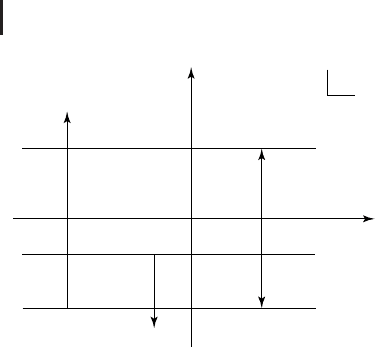
240 7 Wiener–Hopf Method and Wiener–Hopf Integral Equation

=−

+ε

=−

Fig. 7.9 Region of analyticity of

−

(k),

(k), and

K(k).

−

(k) is analytic in the lower half plane,

Im k < −a + ε.

(k) is analytic in the upper half plane,

Im k > −a.

K(k) is analytic inside the strip, −a < Im k < b.

Thus

(k) is analytic in the upper half plane,

Im k = k

> −a.

To summarize, we know



φ(x) → e

(a−ε)x

as x →∞,

ψ(x) → e

as x →−∞.

(7.2.10)

Hencewehave

−

(k) =



+∞

dxe

−ikx

φ(x)analyticfor Imk = k

< −a + ε, (7.2.11a)

(k) =



−∞

dxe

−ikx

ψ(x)analyticforImk = k

> −a. (7.2.11b)

Various regions of the analyticity are drawn in Figure 7.9.

Recalling Eq. (7.2.7), we write 1 −λ

K(k) as the ratio of the −function and

the +function,

1 −λ

K(k) = Y

−

(k)/Y

(k). (7.2.12)

From Eqs. (7.2.7) and (7.2.12), we have

−

(k)

−

(k) =−Y

(k)

(k) ≡ F(k), (7.2.13)

where F(k) is an entire function. The asymptotic behavior of F(k)as



→∞will

determine F(k) completely.

7.2 Homogeneous Wiener–Hopf Integral Equation of the Second Kind 241

We know that

−

(k) → 0as



→∞,

(k) → 0as



→∞,

K(k) → 0as



→∞.

(7.2.14)

By Eq. (7.2.12), we know then

−

(k)/Y

(k) → 1, as



→∞. (7.2.15)

We only need to know the asymptotic behavior of Y

−

(k)orY

(k)as



→∞in

order to determine the entire function F(k). Once F(k) is determined, we have from

Eq. (7.2.13)

−

(k) = F(k)/Y

−

(k) (7.2.16)

and we are done.

We remark that it is convenient to choose a function Y

−

(k) which is not only

analytic in the lower half plane but also has no zeros in the lower half plane, so that

F(k)/Y

−

(k)isitselfa− function for all entire F(k). Otherwise, we need to choose

F(k) so as to have zeros exactly at zeros of Y

−

(k) to cancel the possible poles in

F(k)/Y

−

(k) and yield the − function

−

(k).

The factorization of 1 −λ

K(k) is essential in solving the Wiener–Hopf integral

equation of the second kind. As noted earlier, it can be done either by inspection

or by the general method based on the Cauchy integral formula. As a general rule,

we assign

Any pole in the lower half plane (k = p

)toY

(k),

Any zero in the lower half plane (k = z

)toY

(k),

Any pole in the upper half plane (k = p

)toY

−

(k),

Any zero in the upper half plane (k = z

)toY

−

(k).

(7.2.17)

We ﬁrst solve the following simple example where the factorization is carried out

by inspection and illustrate the rational of this general rule for the assignment.

 Example 7.3. Solve

φ(x) = λ



+∞

−

x−y

φ(y)dy, x ≥ 0. (7.2.18)

Solution. Deﬁne

ψ(x) = λ



+∞

−

x−y

φ(y)dy, x < 0. (7.2.19)

242 7 Wiener–Hopf Method and Wiener–Hopf Integral Equation

Also, deﬁne

φ(x) =



φ(x)forx ≥ 0,

0forx < 0.

Take the Fourier transform of Eqs. (7.2.18) and (7.2.19) and add the results together

to obtain

−

(k) +

(k) = λ ·

+ 1

−

(k). (7.2.20)

Now,

K(x) = e

−

→



−x

as x →∞,

as x →−∞.

(7.2.21)

Therefore, φ(y) can be allowed to grow as fast as e

(1−ε)y

as y →∞.Thus

−

(k)is

analytic for k

< −1 +ε.Wealsoﬁndthatψ (x) → e

as x →−∞.Thus

(k)is

analytic for k

> −1.

To solve Eq. (7.2.20), we ﬁrst write

+ 1 −2λ

+ 1

−

(k) =−

(k), (7.2.22)

and then decompose

+ 1 −2λ

+ 1

(7.2.23)

into a ratio of a − function to a + function. The common region of analyticity of

−

(k),

(k), and

K(k) of this example is drawn in Figure 7.10.

The designations, the lower half plane, and the upper half plane, are to be made

relative to a line with

−1 < Im k = k

< −1 +ε. (7.2.24)

Referring to Eq. (7.2.23),

+ 1 = (k + i)(k − i)

so that k = i is a pole of Eq. (7.2.23) in the upper half plane and k =−i is a pole of

Eq. (7.2.23) in the lower half plane. Now look at the numerator of Eq. (7.2.23),

+ 1 −2λ.

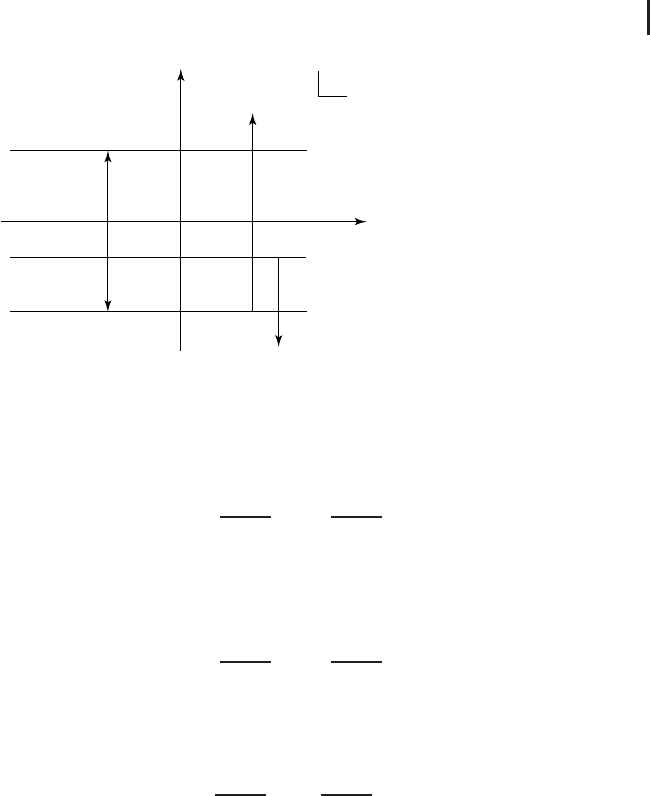
7.2 Homogeneous Wiener–Hopf Integral Equation of the Second Kind 243

= 1

=−1+e

=−1

Fig. 7.10 Common region of analyticity of

−

(k),

and

K(k) of Example 7.3.

−

(k) is analytic in the lower

half plane, Im k < −1 + ε.

(k) is analytic in the upper

half plane, Im k > −1.

K(k) is analytic inside the strip,

−1 < Im k < 1.

Case 1. λ<0. ⇒ 1 −2λ>1.

+ 1 −2λ = (k + i

√

1 −2λ)(k − i

√

1 −2λ). (7.2.25)

The ﬁrst factor corresponds to a zero in the lower half plane, while the second

factor corresponds to a zero in the upper half plane.

Case 2. 0 <λ<1/2. ⇒ 0 < 1 −2λ<1.

+ 1 −2λ = (k + i

√

1 −2λ)(k − i

√

1 −2λ). (7.2.26)

Both factors correspond to a zero in the upper half plane.

Case 3. λ>1/2. ⇒ 1 −2λ<0.

+ 1 −2λ = (k +

√

2λ − 1)(k −

√

2λ − 1). (7.2.27)

Both factors correspond to a zero in the upper half plane.

Now, in general, when we write

1 −λ

K(k) = Y

−

(k)/Y

(k),

since we will end up with

−

(k)

−

(k) =−Y

(k)

(k) ≡ G(k),

which is entire, we wish to have

−

(k) = G(k)/Y

−

(k)

244 7 Wiener–Hopf Method and Wiener–Hopf Integral Equation

analytic in the lower half plane. So, Y

−

(k) must not have any zeros in the lower

half plane. Hence assign any zeros or poles in the lower half plane to Y

(k)sothat

−

(k) has neither poles nor zeros in the lower half plane.

Presently we have

1 −λ

K(k) = (k

+ 1 −2λ)/(k

+ 1)

= (k + i

√

1 −2λ)(k − i

√

1 −2λ)/(k + i)(k − i).

Case 1. λ<0.

k + i

√

1 −2λ ⇒ zero in the lower half plane ⇒ Y

(k)

k − i

√

1 −2λ ⇒ zero in the upper half plane ⇒ Y

−

(k)

k + i ⇒ pole in the lower half plane ⇒ Y

(k)

k − i ⇒ pole in the upper half plane ⇒ Y

−

(k)

Thus we obtain



−

(k) = (k − i

√

1 − 2λ)/(k − i)

(k) = (k + i)/(k + i

√

1 −2λ)

. (7.2.28)

Hence, in the equation

−

(k)

−

(k) =−Y

(k)

(k) = G(k),

we know Y

−

(k) → 1,

−

(k) → 0, as k →∞,sothatG(k) → 0ask →∞.By

Liouville’s theorem , we conclude that G(k) = 0, from which it follows that

−

(k) = 0,

(k) = 0. (7.2.29)

So, there exists no nontrivial solution, i.e.,

φ(x) = 0forλ<0.

Case 2. 0 <λ<1/2.

With a similar analysis as in Case 1, we obtain



−

(k) = (k + i

√

1 − 2λ)(k − i

√

1 −2λ)/(k − i),

(k) = (k + i).

(7.2.30)

Noting that

−

(k) → k as k →∞,

and

−

(k)

−

(k) = G(k),

7.2 Homogeneous Wiener–Hopf Integral Equation of the Second Kind 245

we ﬁnd that G(k) grows less fast than k as k →∞. By Liouville’s theorem, we ﬁnd

G(k) = A,constant,

and thus conclude that

−

(k) = A(k − i)/(k + i

√

1 −2λ)(k − i

√

1 −2λ). (7.2.31)

Case 3. λ>1/2.

With a similar analysis as in Case 1, we obtain



−

(k) = (k +

√

2λ − 1)(k −

√

2λ − 1)/(k − i) → k as k →∞,

(k) = (k + i) → k as k →∞.

(7.2.32)

Again, we ﬁnd that

G(k) = A,constant,

and thus conclude that

−

(k) = A(k − i)/(k +

√

2λ − 1)(k −

√

2λ − 1). (7.2.33)

To summarize, we ﬁnd the following:

λ ≤ 0 ⇒ φ(x) = 0. (7.2.34)

λ>0 ⇒ φ(x) =

2π



dke

ikx

A(k − i)/(k

+ 1 −2λ), (7.2.35)

where the inversion contour C is indicated in Figure 7.11.

For x > 0, we shall close the contour in the upper half plane and get the contribution

from both poles in the upper half plane in either Case 2 or Case 3. The result of

inversions are the following:

Case 2. 0 <λ<1/2.

φ(x) = C



cosh

√

1 −2λx +

sinh

√

1 −2λx

√

1 −2λ



, x > 0. (7.2.36a)

Case 3. λ>1/2.

φ(x) = C



cos

√

2λ − 1x +

sin

√

2λ − 1x

√

2λ − 1



, x > 0. (7.2.36b)

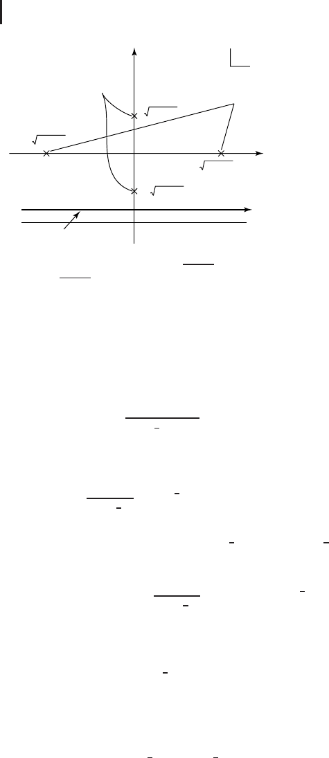
246 7 Wiener–Hopf Method and Wiener–Hopf Integral Equation

−

2l − 1

1 − 2l

−

Case 2

Case 3

Contour C

Fig. 7.11 The inversion contour for φ(x) of Eq. (7.2.35).

Simple poles are located at k =±i

√

1 − 2λ for Case 2 and

at k =±

√

2λ − 1forCase3.

We shall now consider another example where the factorization also is carried out

by inspection after some juggling of the gamma functions.

 Example 7.4. Solve

φ(x) = λ



+∞

cosh[

(x − y)]

φ(y)dy, x ≥ 0. (7.2.37)

Solution. We begin with the Fourier transform of the kernel K(x):

K(x) =

cosh(

x )

→ 2e

−

,as

→∞.

Then

K(k) is analytic inside the strip, −

< Im k = k

.Wecalculate

K(k)as

follows:

K(k) =



+∞

−∞

dxe

−ikx

cosh(

x )

= 2



+∞

−∞

dxe

−ikx

/(e

+ 1).

Setting e

= t, x = ln t, dx = dt/t,wehave

K(k) = 2



+∞

dt[t

−ik−

]/(t + 1).

Further change of variable ρ = 1/(t + 1), t = (1 − ρ)/ρ, dt =−d ρ/ρ

results in

K(k) = 2



dρρ

ik−

(1 −ρ)

−ik−