Mavko G., Mukerji T., Dvorkin J. The Rock Physics Handbook

Подождите немного. Документ загружается.

The alternative V

-only fluid-substitution equations are

ðS

 S

irr

Þ=ð1  S

irr

ð1  S

Þ=ð1  S

irr

mineral

irr

where

¼ M

mineral

M

dry

ð1 þ ÞK

dry

mineral

þ K

ð1  ÞK

þ M

mineral

 K

dry

mineral

irr

¼ M

mineral

M

dry

ð1 þ ÞK

irr

dry

mineral

þ K

irr

ð1  ÞK

irr

þ M

mineral

 K

irr

dry

mineral

Full water saturation (wet rock)

Attenuation is calculated not at a point but in an interval. The necessary condition for

attenuation is elastic heterogeneity in rock. The low-frequency limit of the compres-

sional modulus is calculated by theoretically substituting the pore fluid into the dry-

frame modulus of the spatially averaged rock while the high-frequency modulus is

the spatial average of the saturated-rock modulus. The difference between these two

estimates may give rise to noticeable P-wave attenuation if elastic heterogeneity in

rock is substantial.

Specifically, in an interval of a layered medium, the average porosity is the

arithmetic average of the porosity:



 ¼ 

; the average dry-frame compressional

modulus is the harmonic average of these moduli:

dry

¼ M

1

dry

1

; the average

low-frequency compressional modulus limit is obtained from the V

-only (or, more

rigorously, Gassmann’s) equation applied to these averaged values:

¼ M

mineral





dry

ð1 þ



ÞK

dry

mineral

þ K

ð1 



ÞK



 M

mineral

 K

dry

mineral

where M

mineral

can be estimated by averaging the mineral-component moduli in the

interval by, for example, Hill’s equation or harmonically.

The high-frequency limit is the harmonic average of the wet moduli in the interval:

¼ M

mineral

M

dry

ð1 þ ÞK

dry

mineral

þ K

ð1  ÞK

þ M

mineral

 K

dry

mineral



1

Finally, the inverse P-wave quality factor Q

1

is calculated from the SLS dispersion

equation as presented at the beginning of this section.

Example for wet rock. Consider a model rock that is fully water-saturated (wet) and

has two parts. One part (80% of the rock volume) is shale with porosity 0.4; the clay

content is 0.8 (the rest is quartz); and the P-wave velocity 1.9 km/s. The other part

(the remaining 20%) is clean, high-porosity, slightly-cemented sand with porosity 0.3

and P-wave velocity 3.4 km/s. The compressional modulus is 7 GPa in the shale and

317 6.16 Dvorkin–Mavko attenuation model

25 GPa in the sand. Because of the difference between the compliance of the sand

and shale parts, their deformation due to a passing wave is different, which leads

to macroscopic “squirt-flow.”

At high frequency, there is essentially no cross-flow between sand and shale,

simply because the flow cannot fully develop during the short cycle of oscillation.

The effective elastic modulus of the system is the harmonic (Backus) average of the

moduli of the two parts: M

¼16 GPa.

At low frequency, the cross-flow can easily develop. In this case, the fluid reacts to

the combined deformation of the dry frames of the sand and shale. The dry-frame

compressional modulus in the shale is 2 GPa, while that in the sand is 20 GPa. The

dry-frame modulus of the combined dry frames can be estimated as the harmonic

average of the two: 7 GPa. The arithmetically averaged porosity of the model rock is

0.32. To estimate the effective compressional modulus of the combined dry frame

with water, we theoretically substitute water into this combined frame. The result is

¼13 GPa. The maximum inverse quality factor Q

1

Pmax

is about 0.1 (Q ¼10),

which translates into a noticeable attenuation coefficient 0.05 dB/m at 50 Hz.

At partial saturation, the background inverse quality factor Q

1

Pback

is calculated as if

the entire interval were wet. This value is added to Q

1

PS

which is calculated at partial

saturation (as shown above) to (approximately) arrive at the total inverse quality factor:

1

Ptotal

¼ Q

1

Pback

þ Q

1

PS

An example of applying this model to a pseudo-Earth model is shown in Figure 6.16.1.

0 0.5 1

100

150

200

250

300

Depth (fictitious)

Clay

0 0.5 1

Porosity

1 2 3

and

(km/s)

1.5 2 2.5

Bulk density

(g/cc)

0 0.05 0.1

Figure 6.16.1 A pseudo-Earth model with a relatively fast gas–sand interval embedded in soft shale.

From left to right: clay content; total porosity; velocity; bulk density; the inverse P-wave quality

factor for wet background (dotted curve) and at the actual gas saturation (solid curve); and the

inverse S-wave quality factor.

318 Fluid effects on wave propagation

S-wave attenuation

To model the S-wave inverse quality factor, Dvorkin and Mavko (2006) assume

that the reduction in the compressional modulus between the high-frequency and

low-frequency limits in wet rock is due to the introduction of a hypothetical set of

aligned defects or flaws (e.g., cracks). The same set of defects is responsible for the

reduction in the shear modulus between the high- and low-frequency limits. Finally,

Hudson’s theory for cracked media is used to link the shear-modulus-versus-

frequency dispersion to the compressional-modulus-versus-frequency dispersion

and show that the proportionality coefficient between the two is a function of the

P-to-S-wave velocity ratio (or Poisson’s ratio). This coefficient falls between 0.5

and 3 for Poisson’s ratio contained in the interval 0.25 to 0.35, typical for saturated

Earth materials.

The three proposed versions for Q

1

calculation from Q

1

(as calculated using the

above theory) are:

1

ðM=m  2Þ

ð3M=m  2Þ

ðM=m  1ÞðM=mÞ

1

ðM=m  2Þ

ðM=m  1Þ



2M=m

ð3M=m  2Þ

M=m

3ðM=m  1Þ



1

M=m

ðM=m 

ÞðM=m 

M=m 

where M is the compressional modulus at full water saturation. All three equations

provide results of the same order of magnitude. The result according to the third

equation is displayed in Figure 6.16.1.

Assumptions and limitations

This model estimates fluid-related dispersion and attenuation. The magnitude of

attenuation is estimated as being proportional to the difference between the relaxed

and unrelaxed moduli, using the dispersion–attenuation relation predicted by the

standard linear solid (SLS) model. Choice of the SLS model ignores uncertainty

associated with unknown distributions of fluid relaxation times. For partial saturation,

the unrelaxed modulus is estimated using the patchy saturation model, while the

relaxed modulus is estimated using the fine-scale saturation model. For full water

saturation, the unrelaxed modulus is estimated as the spatial average of point-by-point

Gassmann predictions of saturated moduli, while the relaxed modulus is estimated

from the Gassmann prediction of saturated moduli applied to the spatial average of

dry-rock moduli.

319 6.16 Dvorkin–Mavko attenuation model

6.17 Partial and multiphase saturations

Synopsis

One of the most fundamental observations of rock physics is that seismic velocities

are sensitive to pore fluids. The first-order low-frequency effects for single fluid

phases are often described quite well with Gassmann’s (1951) relations, which are

discussed in Section 6.3. We summarize here variations on those fluid effects that

result from partial or mixed saturations.

Caveat on very dry rocks

Figure 6.17.1 illustrates some key features of the saturation problem. The data are for

limestones measured by Cadoret (1993) using the resonant bar technique at 1 kHz.

The very-dry-rock velocity is approximately 2.84 km/s. Upon initial introduction of

moisture (water), the velocity drops by about 4%. This apparent softening of the rock

occurs at tiny volumes of pore fluid equivalent to a few monolayers of liquid if

distributed uniformly over the internal surfaces of the pore space. These amounts are

hardly sufficient for a fluid dynamic description, as in the Biot–Gassmann theories.

Similar behavior has been reported in sandstones by Murphy (1982), Knight and

Dvorkin (1992), and Tutuncu (1992).

This velocity drop has been attributed to softening of cements (sometimes called

“chemical weakening”), to clay swelling, and to surface effects. In the latter model,

very dry surfaces attract each other via cohesive forces, giving a mechanical effect

resembling an increase in effective stress. Water or other pore fluids disrupt these

forces. A fairly thorough treatment of the subject is found in the articles of Sharma

and Tutuncu (Tutuncu, 1992; Tutuncu and Sharma, 1992; Sharma and Tutuncu, 1994;

Sharma et al., 1994).

After the first few percent of water saturation, additional fluid effects are primarily

elastic and fluid dynamic and are amenable to analysis, for example, by the Biot–

Gassmann (Sections 6.1–6.3) and squirt (Sections 6.10–6.14) models.

Figures 6.17.2 and 6.17.3 (Clark et al., 1980; Winkler and Murphy, 1995) illustrate

further the sensitivity of mechanical properties to very small amounts of water.

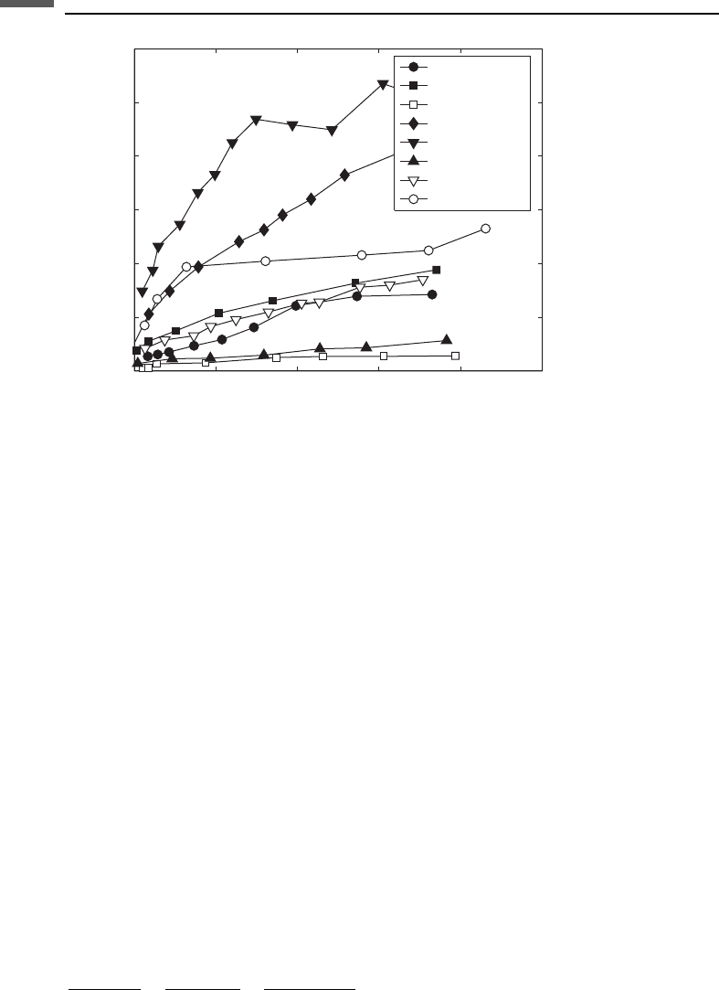
Figure 6.17.2 shows normalized ultrasonic shear-wave velocity in sandstones and

carbonates, plotted versus water vapor partial pressure. In all cases, increased expos-

ure to water molecules systematically decreases the shear stiffness of the rocks, even

though the amount of water is equivalent to only a few monolayers of molecules

coating the pore surfaces. Figure 6.17.3 shows shear-wave attenuation versus water

vapor partial pressure. Attenuation is very small in dry rocks, but increases rapidly

upon expose to moisture.

Several authors (Murphy et al., 1991; Cadoret, 1993) have pointed out that

classical fluid-mechanical models such as the Biot–Gassmann theories perform

320 Fluid effects on wave propagation

poorly when the measured very-dry-rock values are used for the “dry rock” or “dry

frame.” The models can be fairly accurate if the extrapolated “moist” rock modulus

(see Figure 6.17.1) is used instead. For this reason, and to avoid the artifacts of ultra-dry

rocks, it is often recommended to use samples that are at room conditions or that have

been prepared in a constant-humidity environment for measuring “dry-rock” data. For

the rest of this section, it is assumed that the ultra-dry artifacts have been avoided.

Caveat on frequency

It is well known that the Gassmann theory (see Section 6.3) is valid only at

sufficiently low frequencies that the induced pore pressures are equilibrated through-

out the pore space (i.e., that there is sufficient time for the pore fluid to flow and

2.4

2.5

2.6

2.7

2.8

2.9

3.0

0 0.2 0.4 0.6 0.8 1

Limestone – resonant bar

(km/s)

Water saturation

Extrapolated

moist rock

modulus

Very dry rock

Effective fluid

model

(After Cadoret, 1993)

Figure 6.17.1 Extensional-wave velocity versus saturation.

0 0.1 0.2 0.3 0.4 0.5 0.6 0.7 0.8

0.7

0.75

0.8

0.85

0.9

0.95

1.05

O partial pressure

Normalized V

Sioux Qtz

Tennessee Ss

Austin Chalk

Berea Ss

Wingate Ss

Indiana Ls

Boise Ss

Coconino Ss

Figure 6.17.2 Normalized ultrasonic shear-wave velocity versus water partial pressure (Clark et al.,

1980).

321 6.17 Partial and multiphase saturations

eliminate wave-induced pore-pressure gradients). This limitation to low frequencies

explains why Gassmann’s relation works best for very-low-frequency, in-situ seismic

data (< 100 Hz) and may perform less well as frequencies increase toward sonic-

logging (10

Hz) and laboratory ultrasonic measurements (10

Hz). Knight and

Nolen-Hoeksema (1990) studied the effects of pore-scale fluid distributions on

ultrasonic measurements.

Effective fluid model

The most common approach to modeling partial saturation (air/water or gas/water)

or mixed fluid saturations (gas/water/oil) is to replace the collection of phases with

a single “effective fluid.”

When a rock is stressed by a passing wave, pores are always elastically compressed

more than the solid grains. This pore compression tends to induce increments of pore

fluid pressure, which resist the compression; hence, pore phases with the largest bulk

modulus K

stiffen the rock most. For single fluid phases, the effect is described quite

elegantly by Gassmann’s (1951) relation (see Section 6.3):

sat

 K

sat

dry

 K

dry

 K

 K

ðÞ

; m

sat

¼ m

dry

where K

dry

is the effective bulk modulus of the dry rock, K

sat

is the effective bulk

modulus of the rock with pore fluid, K

is the bulk modulus of the mineral material

making up the rock, K

is the effective bulk modulus of the pore fluid, f is porosity,

0 0.2 0.4 0.6 0.8 1

0.005

0.01

0.015

0.02

0.025

0.03

O partial pressure

1/Q

Sioux Qtz

Tennessee Ss

Austin Chalk

Berea Ss

Wingate Ss

Indiana Ls

Boise Ss

Coconino Ss

Figure 6.17.3 Normalized ultrasonic shear-wave attenuation versus water partial pressure

(Clark et al., 1980).

322 Fluid effects on wave propagation

dry

is the effective shear modulus of the dry rock, and m

sat

is the effective shear

modulus of the rock with the pore fluid.

Implicit in Gassmann’s relation is the stress-induced pore pressure

d

1 þ K



1=K

 1=K

ðÞ

1 þ  1=K

 1=K

ðÞ1=K

dry

 1=K



1

where P is the increment of pore pressure and s is the applied hydrostatic stress.

If there are multiple pore-fluid phases with different fluid bulk moduli, then there is

a tendency for each to have a different induced pore pressure. However, when the

phases are intimately mixed at the finest scales, these pore-pressure increments can

equilibrate with each other to a single average value. This is an isostress situation,

and therefore the effective bulk modulus of the mixture of fluids is described well by

the Reuss average (see Section 4.2) as follows:

where K

is the effective bulk modulus of the fluid mixture, K

denotes the bulk

moduli of the individual gas and fluid phases, and S

represents their saturations. The

rock moduli can often be predicted quite accurately by inserting this effective-fluid

modulus into Gassmann’s relation. The effective-fluid (air þ water) prediction is

superimposed on the data in Figure 6.17.1 and reproduces the overall trend quite well.

This approach has been discussed, for example, by Domenico (1976), Murphy

(1984), Cadoret (1993), Mavko and Nolen-Hoeksema (1994), and many others.

Caution

It is thought that the effective-fluid model is valid only when all of the fluid phases

are mixed at the finest scale.

Critical relaxation scale

A critical assumption in the effective-fluid model represented by the Reuss average

is that differences in wave-induced pore pressure have time to flow and equilibrate

among the various phases. As discussed in Section 8.1, the characteristic relaxation

time or diffusion time for heterogeneous pore pressures of scale L is

t 

323 6.17 Partial and multiphase saturations

where D ¼kK

/ is the diffusivity, k is the permeability, K

is the fluid bulk modulus,

and  is the viscosity. Therefore, at a seismic frequency f ¼1/t, pore pressure

heterogeneities caused by saturation heterogeneities will have time to relax and reach

a local isostress state over scales smaller than



ﬃﬃﬃﬃﬃﬃ

ﬃﬃﬃﬃﬃﬃﬃﬃ

D=f

and will be described locally by the effective-fluid model mentioned in the previous

discussion. Spatial fluctuations on scales larger than L

will tend to persist and will

not be described well by the effective-fluid model.

Patchy saturation

Consider the situation of a homogeneous rock type with spatially variable saturation

(x, y, z). Each “patch” or pixel at scale L

will have fluid phases equilibrated

within the patch at scales smaller than L

, but neighboring patches at scales >L

will

not be equilibrated with each other. Each patch will have a different effective fluid

described approximately by the Reuss average. Consequently, the rock in each patch

will have a different bulk modulus describable locally with Gassmann’s relations.

Yet, the shear modulus will remain unchanged and spatially uniform.

The effective moduli of the rock with spatially varying bulk modulus but uniform shear

modulus is described exactly by the equation of Hill (1963) discussed in Section 4.5:

eff

K þ

1



This striking result states that the effective moduli of a composite with uniform shear

modulus can be found exactly by knowing only the volume fractions of the constitu-

ents independent of the constituent geometries. There is no dependence, for example,

on ellipsoids, spheres, or other idealized shapes.

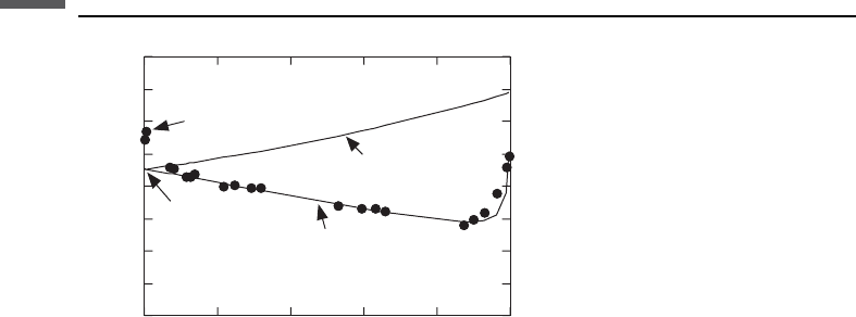
Figure 6.17.4 shows the P-wave velocity versus water saturation for another

limestone (data from Cadoret, 1993). Unlike the effective-fluid behavior, which

shows a small decrease in velocity with increasing saturation and then an abrupt

increase as S

approaches unity, the patchy model predicts a monotonic, almost

linear increase in velocity from the dry to saturated values. The deviation of the data

from the effective-fluid curve at saturations greater than 0.8 is an indication of patchy

saturation (Cadoret, 1993).

The velocity-versus-saturation curves shown in Figure 6.17.4 for the effective-fluid

model and patchy-saturation model represent approximate lower and upper bounds,

respectively, at low frequencies. The lower effective-fluid curve is achieved when the

fluid phases are mixed at the finest scales. The upper patchy-saturation curve is

achieved when there is the greatest separation of phases: when each patch of size >L

324 Fluid effects on wave propagation

has only a single phase. Any velocity between these “bounds” can occur when there is

a range of saturation scales.

Saturation-related velocity dispersion

The difference between effective-fluid behavior and patchy-saturation behavior

is largely a matter of the scales at which the various phases are mixed. The critical-

relaxation scale L

, which separates the two domains, is related to the seismic

frequency. Hence, spatially varying saturations can be a source of velocity dispersion.

Attempts to quantify this velocity dispersion have been made by White (1975) and by

Dutta and Ode

(1979) (see Sections 6.15 and 6.18).

Voigt average approximation

It can be shown that an approximation to the patchy-saturation “upper bound” can be

found by first computing the Voigt average (see Section 4.2) of the fluid modulus:

where K

is the effective bulk modulus of the fluid mixture, K

denotes the bulk

moduli of the individual gas and fluid phases, and S

represents their saturations.

Next, this average fluid is put into Gassmann’s equations to predict the overall rock

moduli. This is in contrast to the effective-fluid model discussed earlier, in which the

Reuss average of the fluid moduli was put into the Gassmann equations.

Brie’s fluid mixing equation

Brie et al. (1995) suggest an empirical fluid mixing law, given by

Brie

¼ðK

liquid

 K

gas

Þð1  S

gas

þ K

gas

2.4

2.5

2.6

2.7

2.8

2.9

3.1

3.2

0 0.2 0.4 0.6 0.8 1

Limestone – resonant bar

(km/s)

Water saturation

Extrapolated

moist rock

modulus

Very dry rock

Effective fluid

model

(After Cadoret, 1993)

Patchy model

Figure 6.17.4 P-wave velocity versus saturation.

325 6.17 Partial and multiphase saturations

where K

gas

is the gas bulk modulus, K

liquid

¼ S

water

þ S

oil

ðÞ

1

is the liquid

bulk modulus given by the Reuss average of the water and oil moduli, K

water

and K

oil

and e is an empirical constant, typically equal to about 3.

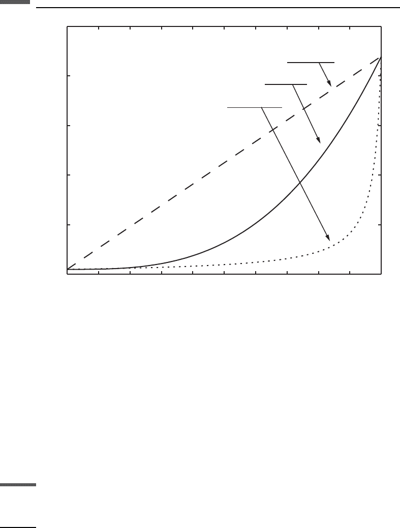
Figure 6.17.5 compares the effective fluid moduli predicted by the Reuss, Voigt,

and Brie averages. While the Voigt and Reuss are bounds for the effective fluid, data

rarely fall near the Voigt average. A more useful range is to assume that the effective

fluid modulus will fall roughly between the Reuss and Brie averages.

6.18 Partial saturation: White and Dutta–Ode

model

for velocity dispersion and attenuation

Synopsis

Consider the situation of a reservoir rock with spatially variable saturation S

(x, y, z).

Each “patch” at scale L

(where L



ﬃﬃﬃﬃﬃﬃ

ﬃﬃﬃﬃﬃﬃﬃﬃ

D=f

is the critical fluid-diffusion

relaxation scale, D ¼kK

/ is the diffusivity, k is the permeability, K

is the fluid

bulk modulus, and  is the viscosity) will have fluid phases equilibrated within the

0 0.1 0.2 0.3 0.4 0.5 0.6 0.7 0.8 0.9 1

0.5

1.5

2.5

Voigt

= S

water

+ S

oil

+ S

gas

1/K

Reuss

= S

water

+ S

oil

+ S

gas

Brie

= (K

liquid

– K

gas

)(1 – S

gas

)

+ K

gas

Reuss

Brie

Voigt

Fluid bulk modulus (GPa)

Figure 6.17.5 Comparison of effective fluid moduli, governed by the following equations: Brie’s

patchy mixer (solid line), K

Brie

¼ K

liquid

 K

gas



1  K

gas



þK

gas

; patchy mix Voigt average

(dashed line), K

Voigt

¼ S

water

þ S

oil

þ S

gas

; and fine-scale mix Reuss average

(dotted line), 1=K

Reuss

¼ S

water

þ S

oil

þ S

gas

326 Fluid effects on wave propagation