McConnell Campbell R., Brue Stanley L., Barbiero Thomas P. Microeconomics. Ninth Edition
Подождите немного. Документ загружается.


Column 3 shows the marginal product (MP), the change in total product associ-
ated with each additional unit of labour. Note that with no labour input, total prod-
uct is zero; a plant with no workers will produce no output. The first three units of
labour reflect increasing marginal returns, with marginal products of 10, 15, and 20
units, respectively. But beginning with the fourth unit of labour, marginal product
diminishes continually, becoming zero with the seventh unit of labour and negative
with the eighth.
Average product, or output per labour unit, is shown in column 4. It is calculated
by dividing total product (column 2) by the number of labour units needed to pro-
duce it (column 1). At five units of labour, for example, AP is 14 (= 70/5).
GRAPHICAL PORTRAYAL
Figure 8-2 (Key Graph) shows the diminishing returns data in Table 8-1 graphically
and further clarifies the relationships between total, marginal, and average prod-
ucts. (Marginal product in Figure 8-2(b) is plotted halfway between the units of
labour, since it applies to the addition of each labour unit.)
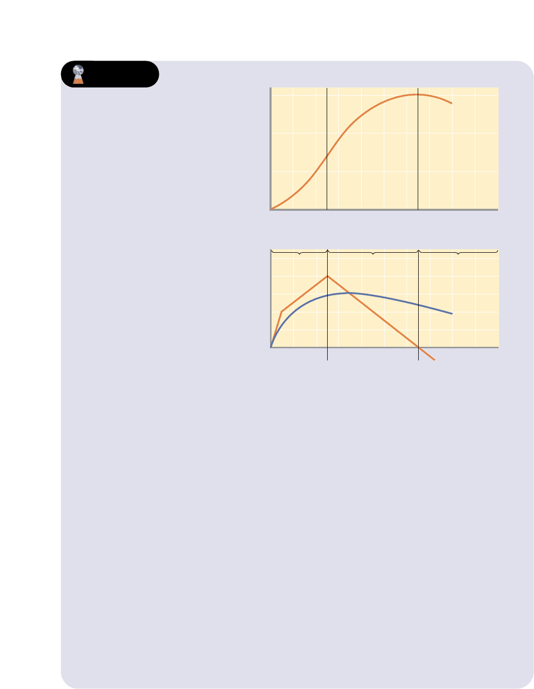
Note first in Figure 8-2(a) that total product, TP, goes through three phases: it rises
initially at an increasing rate; then it increases, but at a diminishing rate; finally, after
reaching a maximum, it declines.
Geometrically, marginal product—shown by the MP curve in Figure 8-2(b)—is
the slope of the total product curve. Marginal product measures the change in total
product associated with each succeeding unit of labour. Thus, the three phases of
total product are also reflected in marginal product. Where total product is increas-
ing at an increasing rate, marginal product is rising. Here, extra units of labour are
adding larger and larger amounts to total product. Similarly, where total product is
increasing but at a decreasing rate, marginal product is positive but falling. Each
additional unit of labour adds less to total product than did the previous unit. When
total product is at a maximum, marginal product is zero. When total product
declines, marginal product becomes negative.
Average product, AP in Figure 8-2(b), displays the same tendencies as marginal
product. It increases, reaches a maximum, and then decreases as more units of
labour are added to the fixed plant. Note the relationship between marginal prod-
uct and average product: Where marginal product exceeds average product, aver-
age product rises, and where marginal product is less than average product, average
product declines. It follows that marginal product intersects average product where
average product is at a maximum.
This relationship is a mathematical necessity. If you add a larger number to a total
than the current average of that total, the average must rise; if you add a smaller
number to a total than the current average of that total, the average must fall. You
raise your average examination grade only when your score on an additional (mar-
ginal) examination is greater than the average of all your past scores. You lower
your average when your grade on an additional exam is below your current aver-
age. In our production example, when the amount an extra worker adds to total
product exceeds the average product of all workers currently employed, average
product will rise. Conversely, when an extra worker adds to total product an
amount that is less than the current average product, then average product will
decrease.
The law of diminishing returns is embodied in the shapes of all three curves. But,
as our definition of the law of diminishing returns indicates, economists are most
concerned with its effects on marginal product. The regions of increasing, dimin-
ishing, and negative marginal product (returns) are shown in Figure 8-2(b). (Key
Question 6)
190 Part Two • Microeconomics of Product Markets
chapter eight • the organization and the costs of production 191
75
50
25
0123456789
Total product, TP
Quantity of labour
(a) Total product
TP
0 123456789
Marginal product, MP
Quantity of labour
(b) Marginal and average product
MP
Increasing
marginal
returns
Diminishing marginal
returns
Negative
marginal
returns
20
10
AP
Panel (a): As a variable resource
(labour) is added to fixed amounts of
other resources (land or capital), the
total product that results will eventu-
ally increase by diminishing amounts,
reach a maximum, and then decline.
Panel (b): Marginal product is the
change in total product associated
with each new unit of labour. Average
product is simply output per labour
unit. Note that marginal product
intersects average product at the
maximum average product.
FIGURE 8-2 THE LAW OF DIMINISHING RETURNS
Key Graph
Quick Quiz
1. Which of the following is an assumption underlying these figures?
a. Firms first hire highly skilled workers and then hire less skilled workers.
b.
Capital and labour are both variable, but labour increases more rapidly than capital.
c. Consumers will buy all the output (total product) produced.
d. Workers are of equal quality.
2. Marginal product is
a. the change in total product divided by the change in the quantity of labour.
b. total product divided by the quantity of labour.
c. always positive.
d. unrelated to total product.
3. Marginal product in graph (b) is zero when
a. average product in graph (b) stops rising.
b. the slope of the marginal-product curve in graph (b) is zero.
c. total product in graph (a) begins to rise at a diminishing rate.
d. the slope of the total-product curve in graph (a) is zero.
4. Average product in graph (b)
a. rises when it is less than marginal product.
b. is the change in total product divided by the change in the quantity of labour.
c. can never exceed marginal product.
d. falls whenever total product in graph (a) rises at a diminishing rate.
Answers
1. d; 2. a; 3. d; 4. a

Production information such as that provided in Table 8-1 and Figure 8-2(a) and (b)
must be coupled with resource prices to determine the total and per-unit costs of
producing various levels of output. We know that in the short run some resources,
those associated with the firm’s plant, are fixed. Others resource, however, are vari-
able. So short-run costs are either fixed or variable.
Fixed, Variable, and Total Cost
Let’s see what distinguishes fixed costs, variable costs, and total costs from one
another.
FIXED COSTS
Fixed costs are those costs that in total do not vary with changes in output. Fixed costs
are associated with the very existence of a firm’s plant and, therefore, must be paid
even if its output is zero. Such costs as rental payments, interest on a firm’s debts, a
portion of depreciation on equipment and buildings, and insurance premiums are
generally fixed costs; they do not increase even if a firm produces more. In column
2 in Table 8-2 we assume that the firm’s total fixed cost is $100. By definition, this
fixed cost is incurred at all levels of output, including zero. The firm cannot avoid
paying these costs in the short run.
VARIABLE COSTS
Variable costs are those costs that change with the level of output. They include pay-
ments for materials, fuel, power, transportation services, most labour, and similar
variable resources. In column 3 of Table 8-2 we find that the total of variable costs
changes directly with output, but note that the increases in variable cost associated
with succeeding one-unit increases in output are not equal. As production begins,
variable cost will for a time increase by a decreasing amount; this is true through the
fourth unit of output in Table 8-2. Beyond the fourth unit, however, variable cost
rises by increasing amounts for succeeding units of output.
The reason lies in the shape of the marginal product curve. At first, as in Figure
8-2(b), marginal product is increasing, so smaller and smaller increases in the
amounts of variable resources are needed to produce successive units of output.
Hence the variable cost of successive units of output decreases. But when, as dimin-
ishing returns are encountered, marginal product begins to decline, larger and
larger additional amounts of variable resources are needed to produce successive
units of output. Total variable cost, therefore, increases by increasing amounts.
TOTAL COST
Total cost is the sum of fixed cost and variable cost at each level of output. It is shown in
column 4 in Table 8-2. At zero units of output, total cost is equal to the firm’s fixed
cost. Then for each unit of the 10 units of production, total cost increases by the same
amount as variable cost.
Figure 8-3 shows graphically the fixed-cost, variable-cost, and total-cost data
given in Table 8-2. Observe that total variable cost, TVC, is measured vertically from
the horizontal axis at each level of output. The amount of fixed cost, shown as TFC,
is added vertically to the total variable cost curve to obtain the points on the total-
cost curve, TC.
192 Part Two • Microeconomics of Product Markets
Short-Run Production Costs
fixed costs
Costs that in total
do not change when
the firm changes its
output; the costs of
fixed resources.
variable
costs
Costs
that in total increase
when the firm
increases its output
and decrease
when it reduces
its output.
total cost
The sum of fixed
cost and variable
cost.

chapter eight • the organization and the costs of production 193
TABLE 8-2 TOTAL-COST, AVERAGE-COST, AND MARGINAL-COST
SCHEDULES FOR AN INDIVIDUAL FIRM IN THE
SHORT RUN
TOTAL-COST DATA AVERAGE-COST DATA MARGINAL COST
(1) (2) (3) (4) (5) (6) (7) (8)
Total Total Total Total Average Average Average Marginal
product fixed variable cost (TC) fixed cost variable total cost cost (MC)
(Q) cost (TFC) cost (TVC) (AFC) cost (AVC) (ATC)
TC = TFC
AFC = AVC = ATC = MC =
+ TVC
0 $100 $ 0 $ 100
1 100 90 190 $100.00 $90.00 $190.00
$90
2 100 170 270 50.00 85.00 135.00
80
3 100 240 340 33.33 80.00 113.33
70
4 100 300 400 25.00 75.00 100.00
60
5 100 370 470 20.00 74.00 94.00
70
6 100 450 550 16.67 75.00 91.67
80
7 100 540 640 14.29 77.14 91.43
90
8 100 650 750 12.50 81.25 93.75
110
9 100 780 880 11.11 86.67 97.78
130
10 100 930 1030 10.00 93.00 103.00
150
change in TC
ᎏᎏ
change in Q
TC
ᎏ
Q
TVC
ᎏ
Q
TFC
ᎏ
Q
FIGURE 8-3 TOTAL COST IS THE SUM OF FIXED COST AND
VARIABLE COST
$1,100
1,000
900
800
700
600
500
400
300
200
100
0 12345678910
Q
Fixed cost
Variable cost
Total
cost
Costs
TC
TVC
TFC
Total variable cost
(TVC) changes with
output. Total fixed
cost (TFC) is inde-
pendent of the level
of output. The total
cost (TC) at any out-
put is the vertical
sum of the fixed cost
and variable cost at
that output.
The distinction between fixed and variable costs is significant to the business
manager. Variable costs can be controlled or altered in the short run by changing
production levels. Fixed costs are beyond the business manager’s current control;
they are incurred in the short run and must be paid regardless of output level.
Per-Unit, or Average, Costs
Producers are certainly interested in their total costs, but they are equally concerned
with per-unit, or average, costs. In particular, average-cost data are more meaning-
ful for making comparisons with product price, which is always stated on a per-unit
basis. Average fixed cost, average variable cost, and average total cost are shown in
columns 5 to 7, Table 8-2.
AFC
Average fixed cost (AFC) for any output level is found by dividing total fixed cost
(TFC) by that output (Q). That is,
AFC =
Because the total fixed cost is, by definition, the same regardless of output, AFC
must decline as output increases. As output rises, the total fixed cost is spread over
a larger and larger output. When output is just one unit in Table 8-2, TFC and AFC
are the same at $100. But at two units of output, the total fixed cost of $100 becomes
$50 of AFC or fixed cost per unit; then it becomes $33.33 per unit as $100 is spread
over three units, and $25 per unit when spread over four units. This process is some-
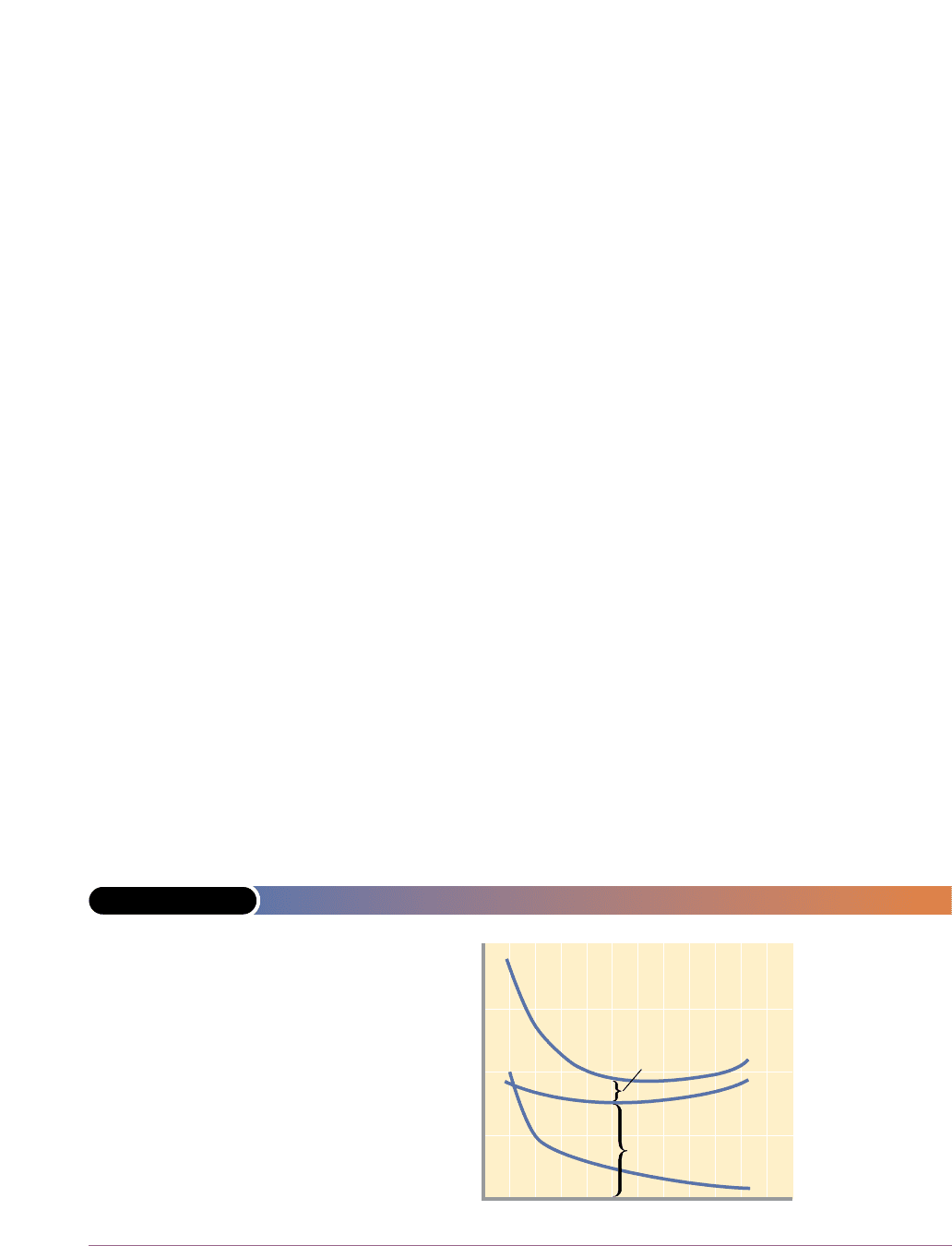
times referred to as “spreading the overhead.” Figure 8-4 shows that AFC graphs as
a continuously declining curve as total output is increased.
AVC
Average variable cost (AVC) for any output level is calculated by dividing total
variable cost (TVC) by that output (Q):
AVC =
TVC
ᎏ
Q
TFC
ᎏ
Q
194 Part Two • Microeconomics of Product Markets
FIGURE 8-4 THE AVERAGE-COST CURVES
$200
150
100
50
0 1234567 8910
Q
Costs
ATC
AVC
AVC
AFC
AFC
AFC falls as a given
amount of fixed
costs is apportioned
over a larger and
larger output. AVC
initially falls because
of increasing mar-
ginal returns but then
rises because of
diminishing marginal
returns. Average total
cost (ATC) is the ver-
tical sum of average
variable cost (AVC)
and average fixed
cost (AFC).
average
fixed cost
(afc)
A firm’s
total fixed cost
divided by output
(the quantity of
product produced).
average
variable
cost (avc)
A
firm’s total variable
cost divided by out-
put (the quantity of
product produced).

As added variable resources increase output, AVC declines initially, reaches a
minimum, and then increases again. A graph of AVC is a U-shaped or saucer-shaped
curve, as shown in Figure 8-4.
Because total variable cost reflects the law of diminishing returns, so must AVC,
which is derived from total variable cost. Because marginal returns increase initially,
it takes fewer and fewer additional variable resources to produce each of the first
four units of output. As a result, variable cost per unit declines. AVC hits a minimum
with the fifth unit of output, and beyond that point AVC rises as diminishing
returns require more variable resources to produce each additional unit of output.
In simpler terms, at very low levels of output, production is relatively inefficient
and costly. Because the firm’s fixed plant is understaffed, average variable cost is rel-
atively high. As output expands, however, greater specialization and better use of
the firm’s capital equipment yield more efficiency, and variable cost per unit of out-
put declines. As still more variable resources are added, a point is reached when
diminishing returns are incurred. The firm’s capital equipment is now staffed more
intensively, and, therefore, each added input unit does not increase output by as
much as preceding inputs, which means that AVC eventually increases.
You can verify the U or saucer shape of the AVC curve by returning to Table 8-1.
Assume the price of labour is $10 per unit. By dividing average product (output per
labour unit) into $10 (price per labour unit), we determine the labour cost per unit
of output. Because we have assumed labour to be the only variable input, the labour
cost per unit of output is the variable cost per unit of output or AVC. When average
product is initially low, AVC is high. As workers are added, average product rises
and AVC falls. When average product is at its maximum, AVC is at its minimum.
Then, as still more workers are added and average product declines, AVC rises. The
hump of the average-product curve is reflected in the saucer or U shape of the AVC
curve. As you will soon see, the two are mirror images.
ATC
Average total cost (ATC) for any output level is found by dividing total cost (TC)
by that output (Q) or by adding AFC and AVC at that output:
ATC = = + = AFC + AVC
Graphically, ATC can be found by adding vertically the AFC and AVC curves, as in
Figure 8-4. Thus, the vertical distance between the ATC and AVC curves measures
AFC at any level of output.
Marginal Cost
One final and very crucial cost concept remains: Marginal cost (MC) is the extra, or
additional, cost of producing one more unit of output. MC can be determined for each
added unit of output by noting the change in total cost that that unit’s production
entails:
MC =
CALCULATIONS
In column 4, Table 8-2 on page 193, production of the first unit of output increases
total cost from $100 to $190. Therefore, the additional, or marginal, cost of that first
unit is $90 (column 8). The marginal cost of the second unit is $80 (= $270 – $190);
change in TC
ᎏᎏ
change in Q
TVC
ᎏ
Q
TFC
ᎏ
Q
TC
ᎏ
Q
chapter eight • the organization and the costs of production 195
average
total cost
(atc)
A firm’s
total cost divided
by output (the quan-
tity of product pro-
duced); equal to
average fixed cost
plus average vari-
able cost.
marginal
cost (mc)
The
extra or additional
cost of producing
one more unit of
output equal to the
change in total cost
divided by the
change in output
(and in the short
run to the change in
total variable cost
divided by the
change in output).
Choosing
a Little More
or Less

the MC of the third is $70 (= $340 – $270); and so forth. The MC for each of the 10
units of output is shown in column 8.
MC can also be calculated from the total-variable-cost column, because the only
difference between total cost and total variable cost is the constant amount of fixed
costs ($100). Thus, the change in total cost and the change in total variable cost asso-
ciated with each additional unit of output are always the same.
MARGINAL DECISIONS
Marginal costs are costs the firm can control directly and immediately. Specifically,
MC designates all the additional cost incurred in producing the last unit of output.
Thus, it also designates the cost that can be saved by not producing that last unit.
Average-cost figures do not provide this information. For example, suppose the firm
is undecided whether to produce three or four units of output. At four units Table 8-2
indicates that ATC is $100. But the firm does not increase its total costs by $100 by
producing the fourth unit, nor does it save $100 by not producing that unit. Rather,
the change in costs involved here is only $60, as the MC column in Table 8-2 reveals.
A firm’s decisions as to what output level to produce are typically marginal deci-
sions, that is, decisions to produce a few more or a few less units. Marginal cost is
the change in costs when one more or one fewer unit of output is produced. When
coupled with marginal revenue (which, as you will see in Chapter 9, indicates the
change in revenue from one more or one fewer unit of output), marginal cost allows
a firm to determine whether it is profitable to expand or contract its production. The
analysis in the next three chapters focuses on those marginal calculations.
GRAPHICAL PORTRAYAL
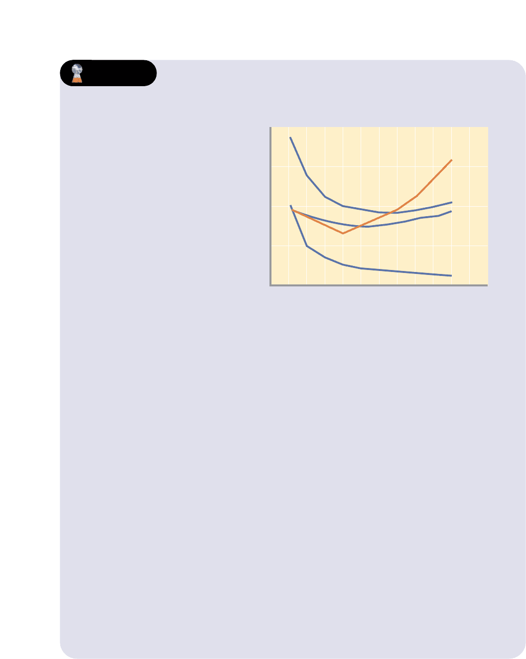
Marginal cost is shown graphically in Figure 8-5 (Key Graph). Marginal cost at first
declines sharply, reaches a minimum, and then rises rather abruptly. This pattern
reflects the fact that the variable costs, and therefore total cost, increase first by decreas-
ing amounts and then by increasing amounts (see columns 3 and 4, Table 8-2).
MC AND MARGINAL PRODUCT
The shape of the marginal-cost curve is a consequence of the law of diminishing
returns. Looking back at Table 8-1, we can see the relationship between marginal
product and marginal cost. If all units of a variable resource (here labour) are hired
at the same price, the marginal cost of each extra unit of output will fall as long as
the marginal product of each additional worker is rising, because marginal cost is
the (constant) cost of an extra worker divided by his or her marginal product. There-
fore, in Table 8-1, suppose that each worker can be hired for $10. Because the first
worker’s marginal product is 10 units of output, and hiring this worker increases
the firm’s costs by $10, the marginal cost of each of these 10 extra units of output is
$1 (= $10 ÷ 10 units). The second worker also increases costs by $10, but the marginal
product is 15, so the marginal cost of each of these 15 extra units of output is $.67
(= $10 ÷ 15 units). Similarly, the MC of each of the 20 extra units of output con-
tributed by the third worker is $.50 (= $10 ÷ 20 units). To generalize, as long as mar-
ginal product is rising, marginal cost will fall.
With the fourth worker, diminishing returns set in and marginal cost begins to
rise. For the fourth worker, marginal cost is $.67 (= $10 ÷ 15 units); for the fifth
worker, MC is $1.00 ($10 ÷ 10 units); for the sixth, MC is $2,00 (= $10 ÷ 5 units), and
so on. If the price (cost) of the variable resource remains constant, increasing mar-
ginal returns will be reflected in a declining marginal cost, and diminishing marginal
196 Part Two • Microeconomics of Product Markets
chapter eight • the organization and the costs of production 197
$200
150
100
50
012
3
4
5
6
7
8910
Q
Quantity
Costs
MC
ATC
AVC
AFC
The marginal-cost (MC) curve cuts
through the average-total-cost (ATC)
curve and the average-variable-cost
(AVC) curve at their minimum points.
When MC is below average total
cost, ATC falls; when MC is above
average total cost, ATC rises.
Similarly, when MC is below average
variable cost, AVC falls; when MC
is above average variable cost,
AVC rises.
FIGURE 8-5 THE RELATIONSHIP OF THE
MARGINAL-COST CURVE TO THE
AVERAGE-TOTAL-COST AND AVERAGE-
VARIABLE-COST CURVES
Key Graph
Quick Quiz
1. The marginal-cost curve first declines and then increases because of
a. increasing, then diminishing, marginal utility.
b. the decline in the gap between ATC and AVC as output expands.
c. increasing, then diminishing, marginal returns.
d. constant marginal revenue.
2. The vertical distance between ATC and AVC measures
a. marginal cost.
b. total fixed cost.
c. average fixed cost.
d. economic profit per unit.
3. ATC is
a. AVC – AFC.
b. MC + AVC.
c. AFC + AVC.
d. (AFC + AVC) × Q.
4. When the marginal-cost curve lies
a. above the ATC curve, ATC rises.
b. above the AVC curve, ATC rises.
c. below the AVC curve, total fixed cost increases.
d. below the ATC curve, total fixed cost falls.
Answers
1. c; 2. c; 3. c; 4. a
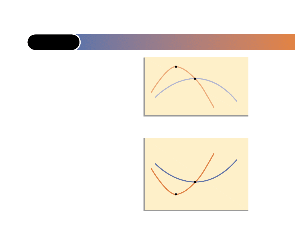
returns in a rising marginal cost. The MC curve is a mirror reflection of the marginal-
product curve. As you can see in Figure 8-6, when marginal product is rising,
marginal cost is necessarily falling. When marginal product is at its maximum, mar-
ginal cost is at its minimum; when marginal product is falling, marginal cost is rising.
RELATION OF MC TO AVC AND ATC
Figure 8-5 shows that the marginal-cost curve MC intersects both the AVC and ATC
curves at their minimum points. As noted earlier, this marginal-average relationship
is a mathematical necessity, which a simple illustration will reveal. Suppose a base-
ball pitcher has allowed his opponents an average of three runs per game in the first
three games he has pitched. Now, whether his average falls or rises as a result of
pitching a fourth (marginal) game will depend on whether the additional runs he
allows in that extra game are fewer or more than his current three-run average. If in
the fourth game he allows fewer than three runs, for example one, his total runs will
rise from 9 to 10 and his average will fall from 3 to 2.5 (= 10 ÷ 4). Conversely, if in
the fourth game he allows more than three runs, say, seven, his total will increase
from 9 to 16 and his average will rise from 3 to 4 (= 16 ÷ 4).
So it is with costs. When the amount (the marginal cost) added to total cost is less
than the current average total cost, ATC will fall. Conversely, when the marginal
cost exceeds ATC, ATC will rise, which means that in Figure 8-5, as long as MC lies
below ATC, ATC will fall, and whenever MC lies above ATC, ATC will rise. At the
198 Part Two • Microeconomics of Product Markets
FIGURE 8-6 THE RELATIONSHIP BETWEEN PRODUCTIVITY
CURVES AND COST CURVES
Average product and
marginal product
Quantity of labour
Quantity of output
Cost (dollars)
0
0
(a) Production curves
(b) Cost curves
AP
MP
MC
AVC
The marginal-cost
(MC) curve and the
average-variable-
cost (AVC) curve in
panel (b) are mirror
images of the mar-
ginal-product (MP)
and average-product
(AP) curves in panel
(a). Assuming that
labour is the only
variable input and
that its price (the
wage rate) is con-
stant, then when
MP is rising, MC is
falling, and when
MP is falling, MC is
rising. Under the
same assumptions,
when AP is rising,
AVC is falling, and
when AP is falling,
AVC is rising.

point of intersection, where MC equals ATC, ATC has just stopped falling but has
not yet begun rising. This point, by definition, is the minimum point on the ATC
curve. The marginal-cost curve intersects the average-total-cost curve at the
ATC curve’s minimum point.
Marginal cost can be defined as the addition either to total cost or to total vari-
able cost resulting from one more unit of output; thus, this same rationale explains
why the MC curve also crosses the AVC curve at the AVC curve’s minimum point.
No such relationship exists between the MC curve and the average-fixed-cost curve,
because the two are not related; marginal cost includes only those costs that change
with output, and fixed costs by definition are those that are independent of output.
(Key Question 9)
Shifts of Cost Curves
Changes in either resource prices or technology will cause costs to change and there-
fore the cost curves to shift. If fixed costs double from $100 to $200, the AFC curve
in Figure 8-5 would shift upward. At each level of output, fixed costs are higher. The
ATC curve would also move upward, because AFC is a component of ATC. The
positions of the AVC and MC curves would be unaltered, because their locations are
based on the prices of variable rather than fixed resources. However, if the price
(wage) of labour or some other variable input rose, AVC, ATC, and MC would rise,
and those cost curves would all shift upward. The AFC curve would remain in place
because fixed costs have not changed. And, of course, reductions in the prices of
fixed or variable resources would reduce costs and product shifts of the cost curve
exactly opposite to those just described.
The discovery of a more efficient technology would increase the productivity of
all inputs, and the cost figures in Table 8-2 would all be lower. To illustrate, if labour
is the only variable input, if wages are $10 per hour, and if the average product is 10
units, then AVC would be $1. But if a technological improvement increases the aver-
age product of labour to 20 units, then AVC will decline to $.50. More generally, an
upward shift in the productivity curves shown in Figure 8-6(a) means a downward
shift in the cost curves portrayed in Figure 8-6(b). (See Global Perspective 8.1.)
chapter eight • the organization and the costs of production 199
8.1
140
130
120
110
90
100
80
70
92 93 94 95 96 99
Index (1992 = 100)
9897
U.S.
Canada
Japan
France
Germany
Italy
U.K.
Source: U.S. Bureau of Labor Statistics,
<www.bls.gov/>.
Relative changes in average
labour costs in manufacturing,
1992–1999, selected nations
Average labour costs (labour costs
per unit of output) are a significant
part of average total costs in most
industries. Average labour costs
have varied widely among nations
at various times in recent years. Other
things equal, higher average labour
costs at each output level result in
higher ATC curves; lower average
labour costs result in lower ATC curves.