McConnell Campbell R., Brue Stanley L., Barbiero Thomas P. Microeconomics. Ninth Edition

Подождите немного. Документ загружается.

($111) and multiplying the difference (per-unit proﬁt of $17.25) by the ﬁrm’s equi-

librium level of output (8). Again we obtain an economic proﬁt of $138 per ﬁrm and

$138,000 for the industry.

GRAPHICAL PORTRAYAL

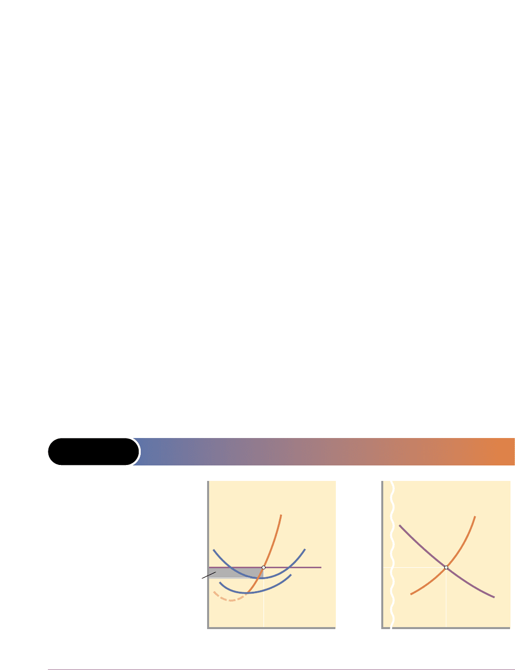
Figure 9-7 shows this analysis graphically. The individual supply curves of each of

the 1000 identical ﬁrms—one of which is shown as s = MC in Figure 9-7(a)—are

summed horizontally to get the total-supply curve S = ∑MC of Figure 9-7(b).

Together with total-demand curve D, it yields the equilibrium price $111 and equi-

librium quantity (for the industry) 8000 units. This equilibrium price is given and

unalterable to the individual ﬁrm; that is, each ﬁrm’s demand curve is perfectly elas-

tic at the equilibrium price, as indicated by d in Figure 9-7(a). Because the individ-

ual ﬁrm is a price-taker, the marginal-revenue curve coincides with the ﬁrm’s

demand curve d. This $111 price exceeds the average total cost at the ﬁrm’s equilib-

rium MR = MC output of eight units, so the ﬁrm earns an economic proﬁt repre-

sented by the grey area in Figure 9-7(a).

Assuming costs or market demand do not change, these diagrams reveal a gen-

uine equilibrium in the short run. The market has no shortages or surpluses to cause

price or total quantity to change. Nor can any one ﬁrm in the industry increase its

proﬁt by altering its output. Note, too, that higher unit and marginal costs on the

one hand, or weaker market demand on the other, could change the situation so that

Figure 9-7(a) resembles Figure 9-4 or Figure 9-5. In Figure 9-7(a) and (b), sketch how

higher costs or decreased demand could produce short-run losses.

FIRM VERSUS INDUSTRY

Figure 9-7 underscores a point made earlier: Product price is a given fact to the indi-

vidual competitive ﬁrm, but the supply plans of all competitive producers as a group

are a basic determinant of product price. If we recall the fallacy of composition,

we ﬁnd there is no inconsistency here. Although one ﬁrm, supplying a negligible

230 Part Two • Microeconomics of Product Markets

FIGURE 9-7 SHORT-RUN COMPETITIVE EQUILIBRIUM FOR A FIRM

(PANEL A) AND THE INDUSTRY (PANEL B)

$111

Economic

profit

$111

0 8,000

(a) Single firm (b) Industry

= MC

ATC

AVC

= ΣMC

The horizontal sum of

the 1000 ﬁrms’ individual

supply curves (s) deter-

mines the industry

supply curve (S). Given

industry demand (D), the

short-run equilibrium

price and output for the

industry are $111 and

8000 units. Taking the

equilibrium price as

given, the individual ﬁrm

establishes its proﬁt-

maximizing output at

eight units and, in this

case, realizes the eco-

nomic proﬁt represented

by the grey area.

fraction of total supply, cannot affect price, the sum of the supply curves of all the

ﬁrms in the industry constitutes the industry supply curve, and that curve does

have an important bearing on price. (Key Question 4)

In the short run a speciﬁc number of ﬁrms are in an industry, each with a ﬁxed, unal-

terable plant. Firms may shut down in the sense that they can produce zero units of

output in the short run, but they do not have sufﬁcient time to liquidate their assets

and go out of business. By contrast, in the long run ﬁrms already in an industry have

sufﬁcient time either to expand or to contract their plant capacities. More important,

the number of ﬁrms in the industry may either increase or decrease as new ﬁrms

enter or existing ﬁrms leave. We now examine how these long-run adjustments

modify our conclusions concerning short-run output and price determination.

Assumptions

We make three simplifying assumptions, none of which affects our conclusions:

1. Entry and exit only The only long-run adjustment is the entry or exit of ﬁrms.

Moreover, we ignore all short-run adjustments to concentrate on the effects of the

long-run adjustments.

chapter nine • pure competition 231

● Proﬁt is maximized, or loss minimized, at the

output at which marginal revenue (or price in

pure competition) equals marginal cost.

● If the market price is below the minimum aver-

age variable cost, the ﬁrm will minimize its

losses by shutting down.

● The segment of the ﬁrm’s marginal-cost curve

that lies above the average-variable-cost curve

is its short-run supply curve.

● Table 9-8 summarizes the MR = MC approach to

determining the competitive ﬁrm’s proﬁt-maxi-

mizing output. It also shows the equivalent

analysis in terms of total revenue and total cost.

● Under competition, equilibrium price is a given

to the individual ﬁrm and simultaneously is the

result of the production (supply) decisions of all

ﬁrms as a group.

TABLE 9-8 OUTPUT DETERMINATION IN PURE COMPETITION

IN THE SHORT RUN

Question Answer

Should this ﬁrm produce? Yes, if price is equal to, or greater than, minimum average variable

cost. This means that the ﬁrm is proﬁtable or that its losses are less

than its ﬁxed cost.

What quantity should this Produce where MR (= P) = MC; there, proﬁt is maximized (TR exceeds

ﬁrm produce? TC by a maximum amount) or loss is minimized.

Will production result in Yes, if price exceeds average total cost (TR will exceed TC). No, if

economic proﬁt? average total cost exceeds price (TC will exceed TR).

Proﬁt Maximization in the Long Run

Identical costs All ﬁrms in the industry have identical cost curves. This assump-

tion lets us discuss an average, or representative, ﬁrm, knowing that all other ﬁrms

in the industry are similarly affected by any long-run adjustments that occur.

3. Constant-cost industry The industry is a constant-cost industry, which means

that the entry or exit of ﬁrms does not affect resource prices or, consequently, the

locations of the average-total-cost curves of individual ﬁrms.

The Goal of Our Analysis

The basic conclusion we want to explain is this: After all long-run adjustments are

completed, product price will be exactly equal to, and production will occur at, each

ﬁrm’s minimum average total cost.

This conclusion follows from two basic facts: (1) Firms seek proﬁts and avoid

losses, and (2) under pure competition, ﬁrms are free to enter and leave an indus-

try. If market price initially exceeds average total costs, the resulting economic prof-

its will attract new ﬁrms to the industry, but this industry expansion will increase

supply until price is brought back down to equality with minimum average total

cost. Conversely, if price is initially less than average total cost, resulting losses will

cause ﬁrms to leave the industry. As they leave, total supply will decline, bringing

the price back up to equality with minimum average total cost.

Long-Run Equilibrium

Consider the average ﬁrm in a purely competitive industry that is initially in long-

run equilibrium. This ﬁrm is represented in Figure 9-8(a), where MR = MC and price

and minimum average total cost are equal at $50. Economic proﬁt here is zero; the

industry is in equilibrium or at rest because there is no tendency for ﬁrms to enter

or to leave. The existing ﬁrms are earning normal proﬁts, which, recall, are included

in their cost curves. The $50 market price is determined in Figure 9-8(b) by market

232 Part Two • Microeconomics of Product Markets

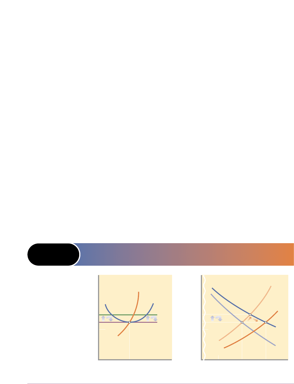
FIGURE 9-8 TEMPORARY PROFITS AND THE RE-ESTABLISHMENT

OF LONG-RUN EQUILIBRIUM IN A REPRESENTATIVE

FIRM (PANEL A) AND THE INDUSTRY (PANEL B)

$60

0 100

$60

0 90,000

100,000 110,000

(a) Single firm (b) Industry

ATC

A favourable shift in

demand (D

to D

) will

upset the original

industry equilibrium

and produce eco-

nomic proﬁts. But

those proﬁts will

cause new ﬁrms to

enter the industry,

increasing supply

to S

) and lower-

ing product price until

economic proﬁts are

once again zero.

or industry demand D

and supply S

. (S

is a short-run supply curve; we will

develop the long-run industry supply curve in our discussion.)

As shown on the quantity axes of the two graphs, equilibrium output in the

industry is 100,000, while equilibrium output for the single ﬁrm is 100. If all ﬁrms

in the industry are identical, there must be 1000 ﬁrms (= 100,000/100).

ENTRY ELIMINATES ECONOMIC PROFITS

Let’s upset the long-run equilibrium in Figure 9-8 and see what happens. Suppose

a change in consumer tastes increases product demand from D

to D

. Price will rise

to $60, as determined at the intersection of D

and S

, and the ﬁrm’s marginal-

revenue curve will shift upward to $60. This $60 price exceeds the ﬁrm’s average

total cost of $50 at output 100, creating an economic proﬁt of $10 per unit. This eco-

nomic proﬁt will lure new ﬁrms into the industry. Some entrants will be newly cre-

ated ﬁrms; others will shift from less prosperous industries.

As ﬁrms enter, the market supply of the product increases, pushing the product

price below $60. Economic proﬁts persist, and entry continues until short-run sup-

ply increases to S

. Market price falls to $50, as does marginal revenue for the ﬁrm.

Price and minimum average total cost are again equal at $50. The economic proﬁts

caused by the boost in demand have been eliminated, and, as a result, the previous

incentive for more ﬁrms to enter the industry has disappeared. Long-run equilib-

rium has been restored.

Observe in Figure 9-8(a) and (b) that total quantity supplied is now 110,000 units

and each ﬁrm is producing 100 units. Now 1100 ﬁrms rather than the original 1000

populate the industry. Economic proﬁts have attracted 100 more ﬁrms.

EXIT ELIMINATES LOSSES

Now let’s consider a shift in the opposite direction. We begin in Figure 9-9(b) with

curves S

and D

setting the same initial long-run equilibrium situation as in our

previous analysis, including the $50 price.

chapter nine • pure competition 233

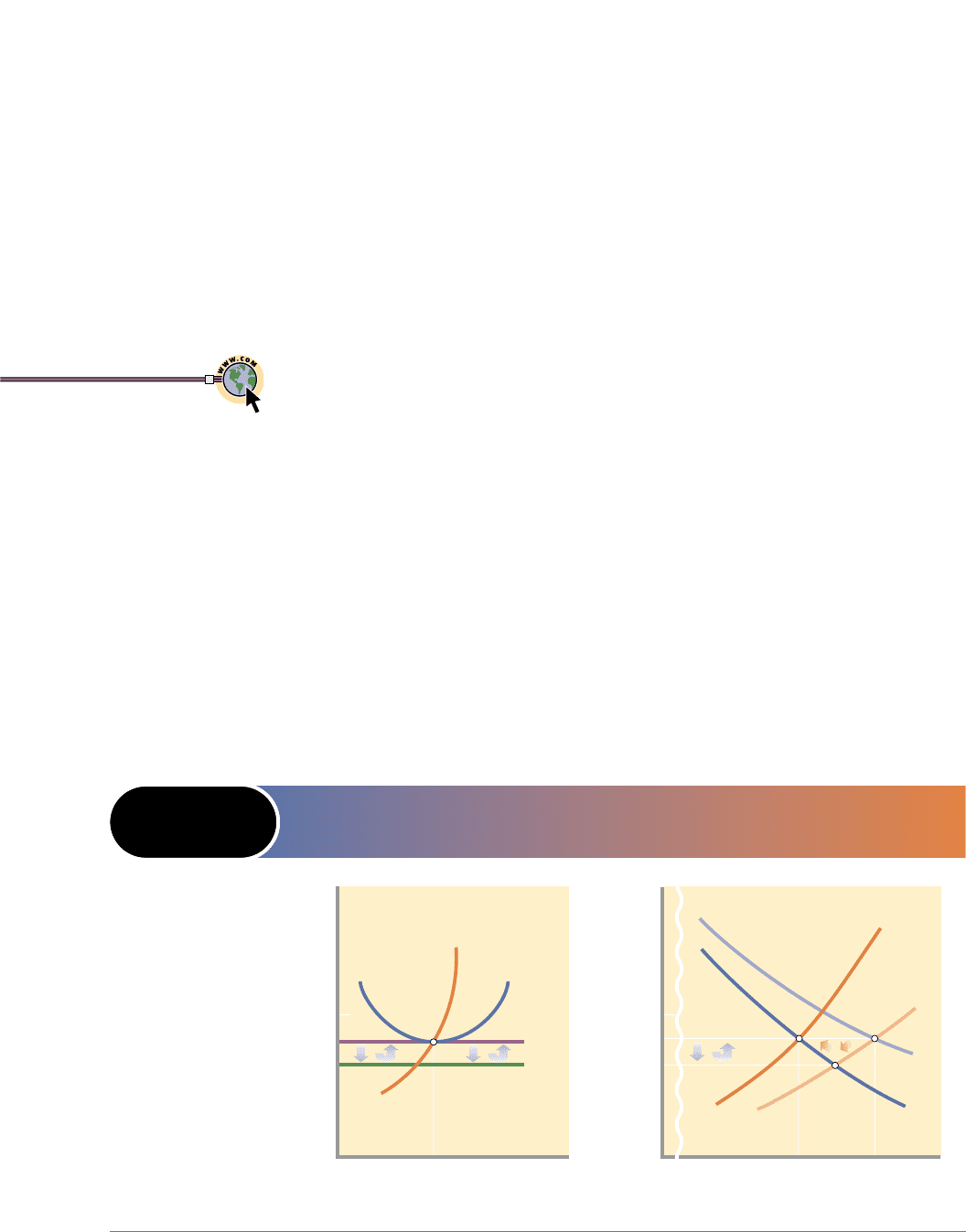
FIGURE 9-9 TEMPORARY LOSSES AND THE RE-ESTABLISHMENT

OF LONG-RUN EQUILIBRIUM IN A REPRESENTATIVE

FIRM (PANEL A) AND THE INDUSTRY (PANEL B)

0 90,000 100,000

$60

0 100

$60

(a) Single firm (b) Industry

ATC

An unfavourable shift

in demand (D

to D

)

will upset the original

industry equilibrium

and produce losses,

but those losses will

cause ﬁrms to leave

the industry, decreas-

ing supply (S

to S

)

and increasing

product price until

all losses have

disappeared.

<economics.about.com/

money/economics/

library/weekly/

aa010900.htm>

The great Pokémon

crash of 2000: Supply

and demand for the

grade school set

Suppose consumer demand declines from D

to D

. This decline forces the mar-

ket price and marginal revenue down to $40, making production unproﬁtable at the

minimum ATC of $50. In time the resulting losses will induce ﬁrms to leave the

industry. Their owners will seek a normal proﬁt elsewhere rather than accept the

below-normal proﬁts (loss) now confronting them. And as capital equipment wears

out, some ﬁrms will simply go out of business. As this exodus of ﬁrms proceeds,

however, industry supply decreases, pushing the price up from $40 toward $50.

Losses continue and more ﬁrms leave the industry until the supply curve shifts to

. Once this happens, price is again $50, just equal to the minimum average total

cost. Losses have been eliminated and long-run equilibrium is restored.

In Figure 9-9(a), total quantity supplied is now 90,000 units and each ﬁrm is pro-

ducing 100 units. Only 900 ﬁrms, not the original 1000, populate the industry.

Losses have forced 100 ﬁrms out.

You may have noted that we have sidestepped the question of which ﬁrms will

leave the industry when losses occur by assuming that all ﬁrms have identical cost

curves. In the real world, of course, entrepreneurial talents differ. Even if resource

prices and technology are the same for all ﬁrms, inferior entrepreneurs tend to incur

higher costs and, therefore, are the ﬁrst to leave an industry when demand declines.

Similarly, ﬁrms with less productive labour forces will be higher-cost producers and

likely candidates to quit an industry when demand decreases.

We have now reached an intermediate goal: Our analysis veriﬁes that competi-

tion, reﬂected in the entry and exit of ﬁrms, eliminates economic proﬁts or losses by

adjusting price to equal minimum long-run average total cost. In addition, this com-

petition forces ﬁrms to select output levels at which average total cost is minimized.

Long-Run Supply for a Constant-Cost Industry

Although our analysis has dealt with the long run, we have noted that the market

supply curves in Figures 9-8(b) and 9-9(b) are short-run curves. What then is the

character of the long-run supply curve of a competitive industry? The analysis

points us toward an answer. The crucial factor here is the effect, if any, that changes

in the number of ﬁrms in the industry will have on costs of the individual ﬁrms in

the industry.

CONSTANT-COST INDUSTRY

In our analysis of long-run competitive equilibrium we assumed that the industry

under discussion was a constant-cost industry, which means that industry expan-

sion or contraction will not affect resource prices or production costs. Graphically,

it means that the entry or exit of ﬁrms does not shift the long-run ATC curves of

individual ﬁrms. This is the case when the industry’s demand for resources is small

in relation to the total demand for those resources; the industry can expand or con-

tract without signiﬁcantly affecting resource prices and costs.

PERFECTLY ELASTIC LONG-RUN SUPPLY

What does the long-run supply curve of a constant-cost industry look like? The

answer is contained in our previous analysis. There we saw that the entry and exit

of ﬁrms changes industry output but always brings the product price back to its

original level, where it is just equal to the constant minimum ATC. Speciﬁcally, we

discovered that the industry would supply 90,000, 100,000, or 110,000 units of out-

put, all at a price of $50 per unit. In other words, the long-run supply of a constant-

cost industry is perfectly elastic.

234 Part Two • Microeconomics of Product Markets

long-run

supply

curve

A curve

that shows the

prices at which a

purely competitive

industry will make

various quantities

of the product avail-

able in the long run.

constant-

cost

industry

industry in which

the entry of new

ﬁrms has no effect

on resource prices

and thus no effect

on production costs.

<www.theshortrun.com/

classroom/

glossary/macro/

marketequilibrium.html>

Market equilibrium

This is demonstrated graphically in Figure 9-10, which uses data from Figures 9-8

and 9-9. Suppose industry demand is originally D

, industry output is Q

(100,000

units), and product price is P

($50). This situation, from Figure 9-8, is one of long-

run equilibrium. We saw that when demand increases to D

, upsetting this equilib-

rium, the resulting economic proﬁts attract new ﬁrms. Because this is a constant-cost

industry, entry continues and industry output expands until the price is driven back

down to the level of the unchanged minimum ATC, which is at price P

($50) and

output Q

(110,000).

From Figure 9-9, we saw that a decline in market demand from D

to D

causes

an exit of ﬁrms and ultimately restores equilibrium at price P

($50) and output Q

(90,000 units). The points Z

, Z

, and Z

in Figure 9-10 represent these three

price–quantity combinations. A line or curve connecting all such points shows the

various price–quantity combinations that ﬁrms would produce if they had enough

time to make all desired adjustments to changes in demand. This line or curve is the

industry’s long-run supply curve. In a constant-cost industry this curve (straight

line) is horizontal, as in Figure 9-10, thus representing perfectly elastic supply.

Long-Run Supply for an Increasing-Cost Industry

Constant-cost industries are a special case. Most industries are increasing-cost

industries, in which ﬁrms’ ATC curves shift upward as the industry expands and

downward as the industry contracts. Usually, the entry of new ﬁrms will increase

resource prices, particularly so in industries using specialized resources whose sup-

plies are not readily increased in response to an increase in resource demand. Higher

resource prices result in higher long-run average total costs for all ﬁrms in the indus-

try. These higher costs cause upward shifts in each ﬁrm’s long-run ATC curve.

Thus, when an increase in product demand results in economic proﬁts and

attracts new ﬁrms to an increasing-cost industry, a two-way squeeze works to elim-

inate those proﬁts. As before, the entry of new ﬁrms increases market supply and

lowers the market price, but now the entire ATC curve shifts upward. The overall

result is a higher-than-original equilibrium price. The industry produces a larger

output at a higher product price because the industry expansion has increased

chapter nine • pure competition 235

FIGURE 9-10 THE LONG-RUN SUPPLY CURVE FOR A CONSTANT-

COST INDUSTRY IS HORIZONTAL

= $50

100,000

110,000

90,000

Because the entry or exodus of

ﬁrms does not affect resource

prices or, therefore, unit costs,

an increase in demand (D

to D

)

causes an expansion in industry

output (Q

to Q

) but no alter-

ation in price ($50). Similarly, a

decrease in demand (D

to D

)

causes a contraction of output

to Q

) but no change in price.

This means that the long-run

industry supply curve (S) is

horizontal through points Z

, Z

and Z

increasing-

cost

industry

industry in which

the entry of new

ﬁrms raises the

prices for resources

and thus increases

their production

costs.

resource prices and the minimum average total cost. We know that, in the long run,

the product price must cover ATC.

Since greater output will be supplied at a higher price, the long-run industry sup-

ply curve is upsloping. Instead of supplying 90,000, 100,000, or 110,000 units at the

same price of $50, an increasing-cost industry might supply 90,000 units at $45,

100,000 units at $50, and 110,000 units at $55. A higher price is required to induce

more production, because costs per unit of output increase as production rises.

We show this in Figure 9-11. Original market demand is D

and industry price

and output are P

($50) and Q

(100,000 units), respectively, at equilibrium point Y

An increase in demand to D

upsets this equilibrium and leads to economic proﬁts.

New ﬁrms enter the industry, increasing both market supply and production costs

of individual ﬁrms. A new price is established at point Y

, where P

is $55 and Q

110,000 units.

Conversely, a decline in demand from D

to D

makes production unproﬁtable

and causes ﬁrms to leave the industry. The resulting decline in resource prices

reduces the minimum average total cost of production for ﬁrms that stay. A new

equilibrium price is established at some level below the original price, say, at point

, where P

is $45 and Q

is 90,000 units. Connecting these three equilibrium posi-

tions, we derive the upsloping long-run supply curve S in Figure 9-11.

Long-Run Supply for a Decreasing-Cost Industry

In a decreasing-cost industry, a ﬁrm experiences lower costs as the industry expands.

The personal computer industry is an example. As demand for personal computers

increased, new manufacturers of computers entered the industry and greatly

increased the resource demand for the components used to build them (for exam-

ple, memory chips, hard drives, monitors, and operating software). The expanded

production of those components enabled the producers of those items to achieve

substantial economies of scale. The decreased production costs of the components

reduced their prices, which greatly lowered the computer manufacturers’ average

costs of production. The supply of personal computers increased by more than

demand, and the price of personal computers declined.

236 Part Two • Microeconomics of Product Markets

FIGURE 9-11 THE LONG-RUN SUPPLY CURVE FOR AN

INCREASING-COST INDUSTRY IS UPSLOPING

$55

100,000

110,000

90,000

In an increasing-cost indus-

try the entry of new ﬁrms in

response to an increase in

demand (D

to D

) will

bid up resource prices and

thereby increase unit costs.

As a result, an increased

industry output (Q

to Q

) will be forthcoming only

at higher prices ($55 > $50 >

$45). The long-run industry

supply curve (S) therefore

slopes upward through

points Y

, Y

, and, Y

decreasing-

cost

industry

industry in which

the entry of ﬁrms

lowers the prices of

resources and thus

decreases produc-

tion costs.

We urge you to rework the analysis underlying Figure 9-11 to show that the long-

run supply curve of a decreasing-cost industry is downsloping. (Key Question 6)

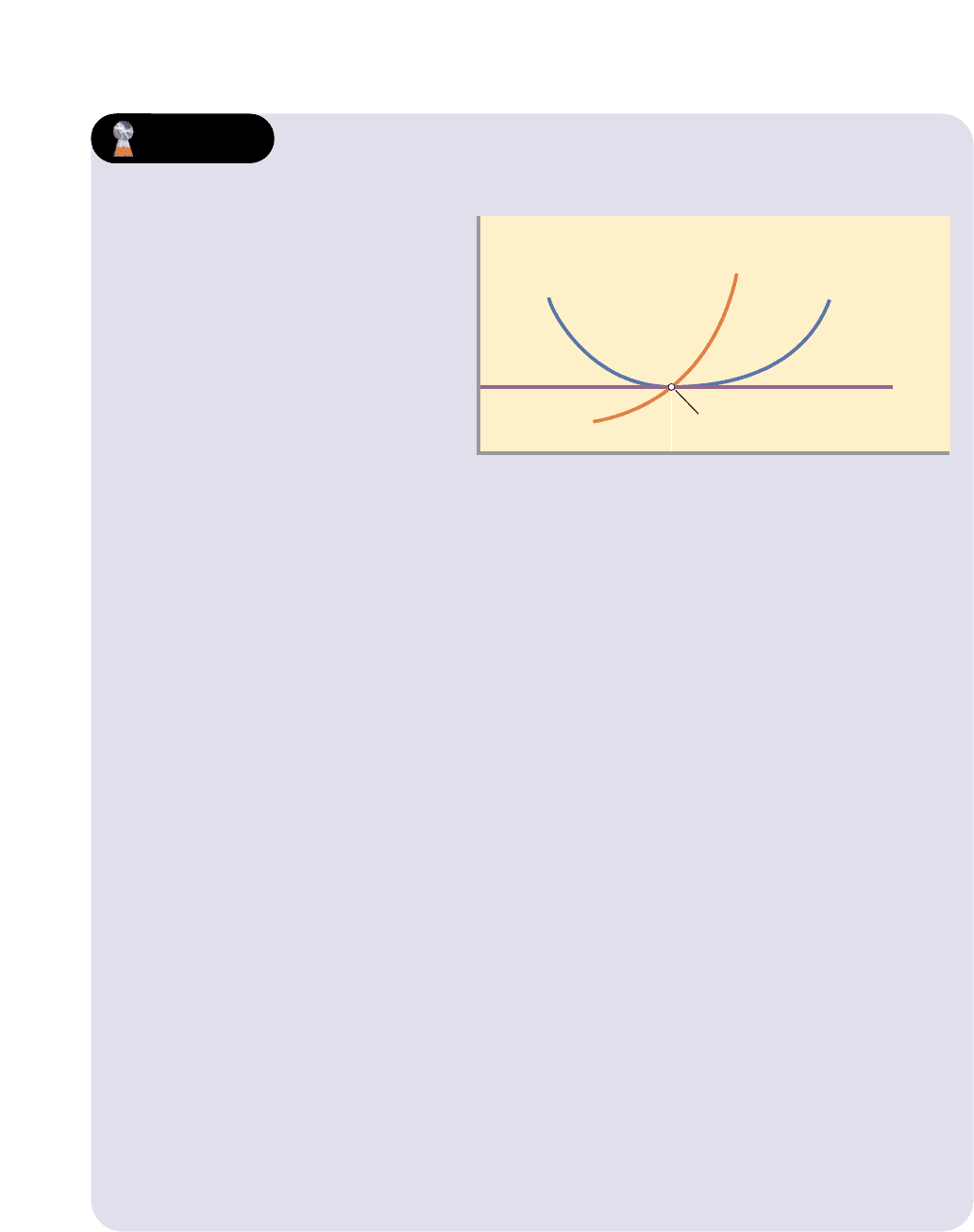
Our ﬁnal goal in this chapter is to relate pure competition to efﬁciency. Whether a

purely competitive industry is a constant-cost industry or an increasing-cost indus-

try, the ﬁnal long-run equilibrium positions of all ﬁrms have the same basic charac-

teristics relating to economic efﬁciency. As shown in Figure 9-12 (Key Graph), price

(and marginal revenue) will settle where it is equal to minimum average total cost:

P (and MR) = minimum ATC. Since the marginal-cost curve intersects the average-

total-cost curve at its minimum point, marginal cost and average total cost are equal:

MC = minimum ATC. Thus, in long-run equilibrium a multiple equality exists: P

(and MR) = MC = minimum ATC.

This triple equality tells us that although a competitive ﬁrm may realize eco-

nomic proﬁt or loss in the short run, it will earn only a normal proﬁt by producing

in accordance with the MR (= P) = MC rule in the long run. Also, this triple equal-

ity suggests certain conclusions of great social signiﬁcance concerning the efﬁ-

ciency of a purely competitive economy.

Economists agree that, subject to qualiﬁcations discussed in later chapters, an

idealized purely competitive economy leads to an efﬁcient use of society’s scarce

resources. A competitive market economy uses the limited amounts of resources

available to society in a way that maximizes the satisfaction of consumers. As we

demonstrated in Chapter 2, efﬁcient use of limited resources requires both produc-

tive efﬁciency and allocative efﬁciency.

Productive efﬁciency requires that goods and services be produced in the least

costly way. Allocative efﬁciency requires that resources be apportioned among

ﬁrms and industries so as to yield the mix of products and services most wanted by

society (consumers). Allocative efﬁciency has been realized when it is impossible to

alter the composition of total output and achieve a net gain for society. Let’s look at

how productive and allocative efﬁciency are achieved under purely competitive

conditions.

Productive Efﬁciency: P = Minimum ATC

In the long run, pure competition forces ﬁrms to produce at the minimum average

total cost of production and to charge a price that is just consistent with that cost, a

highly favourable situation for the consumer. Unless ﬁrms use the best-available

(least-cost) production methods and combinations of inputs, they will not survive.

Stated differently, the minimum amount of resources will be used to produce any

particular output. Let’s suppose that output is cucumbers.

In the ﬁnal equilibrium position shown in Figure 9-9(a), each ﬁrm in the cucum-

ber industry is producing 100 units (say, pickup truckloads) of output by using

$5000 (equal to average total cost of $50 × 100 units) worth of resources. If one ﬁrm

produced that same output at a total cost of, say, $7000, its resources would be used

inefﬁciently. Society would be faced with a net loss of $2000 worth of alternative

products. This loss cannot happen in pure competition; this ﬁrm’s loss of $2000

would require it either to reduce its costs or go out of business.

Note, too, that consumers beneﬁt from productive efﬁciency by paying the low-

est product price possible under the prevailing technology and cost conditions.

chapter nine • pure competition 237

Pure Competition and Efﬁciency

productive

efﬁciency

The production of a

good or service in

the least costly way.

allocative

efﬁciency

When resources are

apportioned among

ﬁrms and industries

to obtain the mix of

products and serv-

ices most wanted

by society.

The

Effectiveness

of Markets

238 Part Two • Microeconomics of Product Markets

= MC = minimum ATC

(normal profit)

Price

Quantity

ATC

The equality of price and minimum

average total cost indicates that the

ﬁrm is using the most efﬁcient

technology, is charging the lowest

price, P, and is producing the great-

est output, Q, consistent with its

costs. The equality of price and mar-

ginal cost indicates that resources

are being allocated in accordance

with consumer preferences.

FIGURE 9-12 THE LONG-RUN EQUILIBRIUM POSITION

OF A COMPETITIVE FIRM: P = MC =

MINIMUM ATC

Key Graph

Quick Quiz

1. We know this ﬁrm is a price-taker because

a. its MC curve slopes upward.

b. its ATC curve is U-shaped.

c. its MR curve is horizontal.

d. MC and ATC are equal at the proﬁt-maximizing output.

2. This ﬁrm’s MC curve is rising because

a. it is a price-taker.

b. of the law of diminishing marginal utility.

c. wage rates rise as output expands.

d. of the law of diminishing marginal returns.

3. At this ﬁrm’s proﬁt-maximizing output

a. total revenue equals total cost.

b. it is earning an economic proﬁt.

c. allocative, but not necessarily productive, efﬁciency is achieved.

d. productive, but not necessarily allocative, efﬁciency is achieved.

4. The equality of P, MC, and minimum ATC

a. occurs only in constant-cost industries.

b. encourages entry of new ﬁrms.

c. means that the right goods are being produced in the right ways.

d. results in a zero accounting proﬁt.

Answers

1. c; 2. d; 3. a; 4. c

Allocative Efﬁciency: P = MC

Productive efﬁciency alone does not ensure the efﬁcient allocation of resources.

Least-cost production must be used to provide society with the right goods—the

goods that consumers want most. Before we can show that the competitive market

system does just that, we must discuss the social meaning of product prices. There

are two critical elements here.

1. The money price of any product is society’s measure of the relative worth of an

additional unit of that product—for example, cucumbers. So, the price of a unit

of cucumbers is the marginal beneﬁt derived from that unit of the product.

2. Similarly, recalling the idea of opportunity cost, we see that the marginal cost of

an additional unit of a product measures the value, or relative worth, of the other

goods sacriﬁced to obtain it. In producing cucumbers, resources are drawn away

from producing other goods. The marginal cost of producing a unit of cucumbers

measures society’s sacriﬁce of those other goods.

To understand why P = MC deﬁnes allocative efﬁciency, let’s ﬁrst look at situations

where that is not the case.

UNDERALLOCATION: P > MC

In pure competition, a ﬁrm will realize the maximum possible proﬁt only by pro-

ducing where price equals marginal cost (Figure 9-12). Producing fewer cucumbers

such that MR (and thus P) exceeds MC yields less than maximum proﬁt. It also

entails, from society’s viewpoint, an underallocation of resources to this product.

The fact that price still exceeds marginal cost indicates that society values additional

units of cucumbers more highly than the alternative products the appropriate

resources could otherwise produce.

To illustrate, if the price or marginal beneﬁt of a unit of cucumbers is $100 and its

marginal cost is $50, producing an additional unit will cause a net increase in total

well-being of $50. Society will gain cucumbers valued at $100, while the alternative

products sacriﬁced by allocating more resources to cucumbers would be valued at

only $50. Whenever society can gain something valued at $100 by giving up some-

thing valued at $50, the initial allocation of resources must have been inefﬁcient.

OVERALLOCATION: P < MC

For similar reasons, the production of cucumbers should not go beyond the output

at which price equals marginal cost. To produce where MC exceeds MR (and thus

P) would yield less than the maximum proﬁt for the producer and, from the view-

point of society, would entail an overallocation of resources to cucumbers. Produc-

ing cucumbers at the level where marginal cost exceeds price (or marginal beneﬁt)

means that society is producing cucumbers by sacriﬁcing alternative goods that

society values more highly.

For example, if the price of a unit of cucumbers is $75 and its marginal cost is

$100, then the production of one less unit of cucumbers would result in a net

increase in society’s total well-being of $25. Society would lose cucumbers valued

at $75, but reallocating the freed resources to their best alternative uses would

increase the output of some other good valued at $100. Whenever society is able to

give up something of lesser value in return for something of greater value, the orig-

inal allocation of resources must have been inefﬁcient.

chapter nine • pure competition 239