McConnell Campbell R., Brue Stanley L., Barbiero Thomas P. Microeconomics. Ninth Edition

Подождите немного. Документ загружается.

So, in practice, it would be difﬁcult to determine how much of any speciﬁc

income payment actually amounted to economic rent.

● So-called unearned income accrues to many people other than landowners,

especially when the economy is growing. For example, consider the capital

gains income received by someone who, some 20 or 25 years ago, chanced to

purchase (or inherit) stock in a ﬁrm that has experienced rapid proﬁt growth.

Is such income more earned than the rental income of the landowner?

● Historically, a piece of land is likely to have changed ownership many times.

Former owners may have been the beneﬁciaries of past increases in the value

of the land (and in land rent). It would hardly be fair to impose a heavy tax on

current owners who paid the competitive market price for the land.

Productivity Differences and Rent Differences

So far we have assumed that all units of land are of the same grade. That is plainly

not so. Different pieces of land vary greatly in productivity, depending on soil fer-

tility and on such climatic factors as rainfall and temperature. Such factors explain,

for example, why Southern Ontario soil is excellently suited to corn production,

why the Prairies are less well suited, and why Yukon is nearly incapable of corn

production. Such productivity differences are reﬂected in resource demand and

prices. Competitive bidding by producers will establish a high rent for highly pro-

ductive Southern Ontario land; less productive Prairie land will command a much

lower rent; and Yukon land may command no rent at all.

Location itself may be just as important in explaining differences in land rent.

Other things equal, renters will pay more for a unit of land that is strategically

located with respect to materials, labour, and customers than they will for a unit of

land whose location is remote from these things. For example, enormously high

land prices are paid for major ski resorts and land that has oil under it.

Figure 16-1, viewed from a slightly different perspective, reveals the rent differ-

entials from quality differences in land. Assume, again, that only wheat can be pro-

duced on four grades of land, each of which is available in the ﬁxed amount L

When combined with identical amounts of labour, capital, and entrepreneurial tal-

ent, the productivity or, more speciﬁcally, the marginal revenue product of each of

the four grades of land is reﬂected in demand curves D

, D

, and D

. Grade 1 land

is the most productive, as shown by D

, while grade 4 is the least productive, as

shown by D

. The resulting economic rents for grades 1, 2, and 3 land will be R

, R

and R

, respectively; the rent differential will mirror the differences in productivity

of the three grades of land. Grade 4 land is so poor in quality that, given its supply

S, farmers won’t pay anything to use it. It will be a free good because it is not sufﬁ-

ciently scarce in relation to the demand for it to command a price or a rent.

Alternative Uses of Land

We have assumed that land has only one use. Actually, we know that land normally

has alternative uses. A hectare of Ontario farmland may be useful for raising not only

corn but also for raising corn, oats, barley, and cattle; or it may be useful for build-

ing a house, or a highway, or as a factory site. In other words, any particular use of

land involves an opportunity cost—the forgone production from the next best use

of the resource. Where there are alternative uses, individual ﬁrms must pay rent to

cover those opportunity costs to secure the use of land for their particular purpose.

To the individual ﬁrm, rent is a cost of production, just as wages and interest are.

chapter sixteen • rent, interest, and proﬁt 421

Recall that, as viewed by society, economic rent is not a cost. Society would have

the same amount of land with or without the payment of economic rent. From soci-

ety’s perspective, economic rent is a surplus payment above that needed to gain the

use of a resource. But individual ﬁrms do need to pay rent to attract land resources

away from alternative uses. For ﬁrms, rental payments are a cost. (Key Question 2)

Interest is the price paid for the use of money. It is the price that borrowers need to pay

lenders for transferring purchasing power from the present to the future. It can be

thought of as the amount of money that must be paid for the use of $1 for one year.

Two points are important to this discussion.

1. Interest is stated as a percentage. Interest is paid in kind; that is, money (inter-

est) is paid for the loan of money. For that reason, interest is typically stated as a

percentage of the amount of money borrowed rather than as a dollar amount. It

is less clumsy to say that interest is “12 percent annually” than to say that inter-

est is “$120 per year per $1000.” Also, stating interest as a percentage makes it

easier to compare the interest paid on loans of different amounts. By expressing

interest as a percentage, we can immediately compare an interest payment of,

say, $432 per year per $2880 with one of $1800 per year per $12,000. Both inter-

est payments are 15 percent per year, which is not obvious from the actual dol-

lar ﬁgures. This interest of 15 percent per year is referred to as a 15 percent

interest rate.

2. Money is not a resource. Money is not an economic resource. In the form of

coins, paper currency, or chequing accounts, money is not productive; it cannot

produce goods and services. However, businesses buy the use of money because

it can be used to acquire capital goods such as factories, machinery, warehouses,

and so on. Such facilities clearly do contribute to production. Thus, in hiring the

use of money capital, business executives are often indirectly buying the use of

real capital goods.

Loanable Funds Theory of Interest

In macroeconomics the interest rate is viewed through the lens of the economy’s

total supply of and demand for money. But since our present focus is on microeco-

nomics, it will be useful to consider a more micro-based theory of interest here.

Speciﬁcally, the loanable funds theory of interest explains the interest rate not in

terms of the total supply of and demand for money but, rather, in terms of supply of

and demand for funds available for lending (and borrowing). As Figure 16-2 shows, the

422 Part Three • Microeconomics of Resource Markets

Interest

● Economic rent is the price paid for resources

such as land whose supply is perfectly inelastic.

● Land rent is a surplus payment because land

would be available to society even if this rent

were not paid.

● The surplus nature of land rent served as the

basis for Henry George’s single-tax movement.

● Differential rents allocate land among alterna-

tive uses.

loanable

funds

theory of

interest

The

concept that the

supply of and de-

mand for loanable

funds determine

the equilibrium rate

of interest.

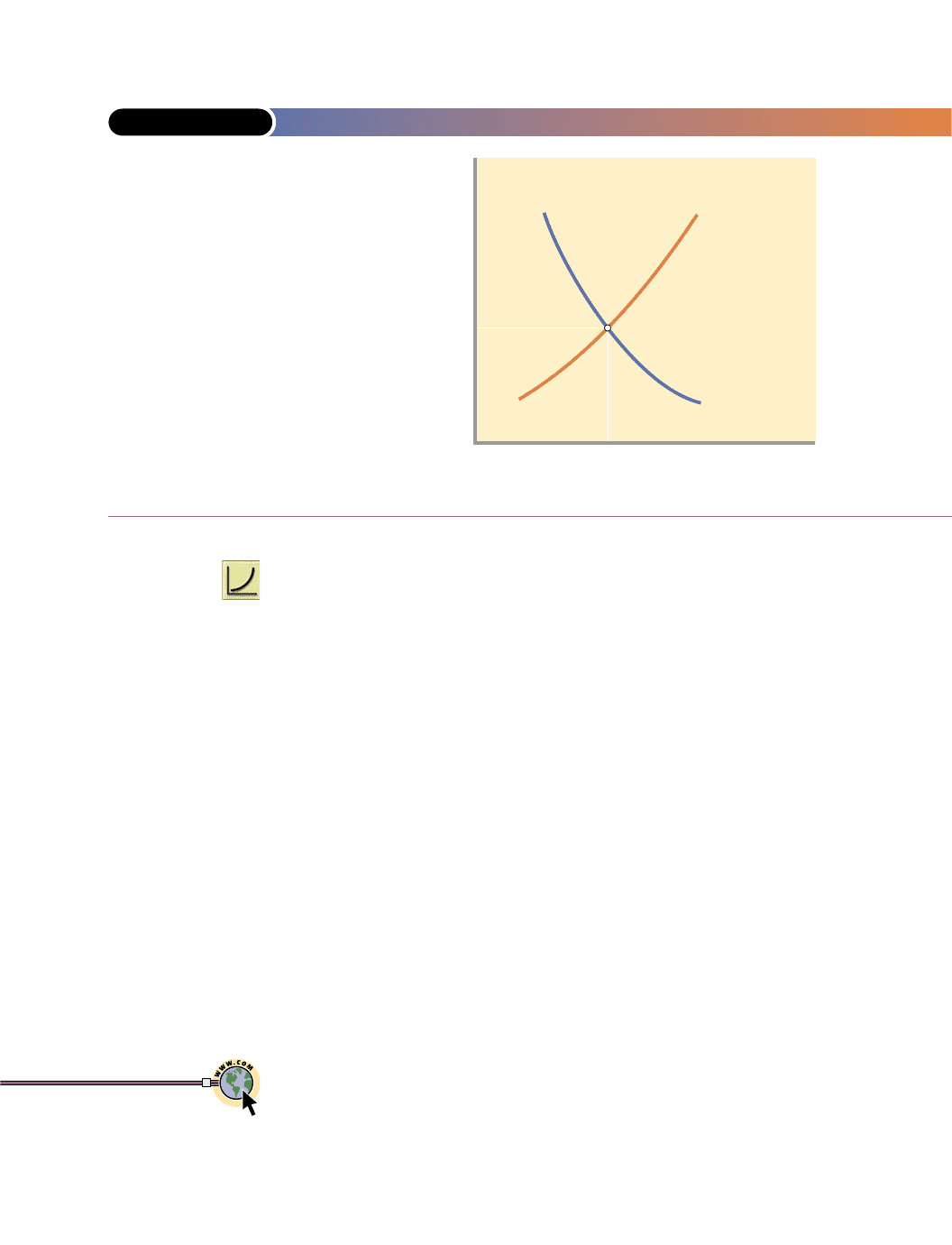
equilibrium interest rate (here, 8 percent) is the rate at which the quantities of loan-

able funds supplied and demanded are equal.

Let’s ﬁrst consider the loanable funds theory in simpliﬁed form. Speciﬁcally,

assume households or consumers are the sole suppliers of loanable funds and busi-

nesses are the sole demanders. Also assume that lending occurs directly between

households and businesses; there are no intermediate ﬁnancial institutions.

SUPPLY OF LOANABLE FUNDS

The supply of loanable funds is represented by curve S in Figure 16-2. Its upward

slope indicates that households will make available a larger quantity of funds at

high interest rates than at low interest rates. Most people prefer to use their income

to purchase pleasurable goods and services today, rather than to delay purchases to

sometime in the future. For people to delay consumption and increase their saving,

they must be compensated by an interest payment. The larger the amount of that

payment, the greater the deferral of household consumption and thus the greater

the amount of money made available for loans.

There is disagreement among economists as to how much the quantity of loan-

able funds made available by suppliers changes in response to changes in the inter-

est rate. Most economists view saving as being relatively insensitive to changes in

the interest rate. The supply curve of loanable funds may, therefore, be more inelas-

tic than S in Figure 16-2 implies.

DEMAND FOR LOANABLE FUNDS

Businesses borrow loanable funds primarily to add to their stocks of capital goods,

such as new plants or warehouses, machinery, and equipment. Assume that a ﬁrm

wants to buy a machine that will increase output and sales such that the ﬁrm’s total

revenue will rise by $110 for the year. Also assume that the machine costs $100 and

has a useful life of just one year. Comparing the $10 earned with the $100 cost of the

machine, we ﬁnd that the expected rate of return on this investment is 10 percent

(= $10/$100) for one year.

chapter sixteen • rent, interest, and proﬁt 423

FIGURE 16-2 THE MARKET FOR LOANABLE FUNDS

Interest rate (percent)

Quantity of loanable funds

The upsloping supply curve

S for loanable funds reﬂects

the idea that at higher inter-

est rates, households will

defer more of their present

consumption (save more),

making more funds available

for lending. The downsloping

demand curve D for loanable

funds indicates that busi-

nesses will borrow more at

lower interest rates than at

higher interest rates. At the

equilibrium interest rate

(here, 8 percent), the quanti-

ties of loanable funds lent

and borrowed are equal

(here, F

each).

<www.mises.com/

humanaction/

chap19sec1.asp>

The phenomenon of

interest

To determine whether the investment would be proﬁtable and whether it should

be made, the ﬁrm must compare the interest rate—the price of loanable funds—with

the 10 percent expected rate of return. If funds can be borrowed at some rate less

than the rate of return, say, at 8 percent, as in Figure 16-2, then the investment is

proﬁtable and should be made. But if funds can be borrowed only at an interest rate

above the 10 percent rate of return, say, at 14 percent, the investment is unproﬁtable

and should not be made.

Why is the demand for loanable funds downsloping, as in Figure 16-2? At higher

interest rates fewer investment projects will be proﬁtable and hence a smaller quan-

tity of loanable funds will be demanded. At lower interest rates, more investment

projects will be proﬁtable and, therefore, more loanable funds will be demanded.

Indeed, as we have just seen, it is proﬁtable to purchase the $100 machine if funds

can be borrowed at 8 percent but not if the ﬁrm must borrow at 14 percent.

Extending the Model

We now make this simple model more realistic in several ways.

FINANCIAL INSTITUTIONS

Households rarely lend their savings directly to businesses that are borrowing

funds for investment. Instead, they place their savings in chartered banks (and other

ﬁnancial institutions). The banks pay interest to savers to attract loanable funds and

in turn lend those funds to businesses. Businesses borrow the funds from the banks,

paying them interest for the use of the money. Financial institutions proﬁt by charg-

ing borrowers higher interest rates than the interest rates they pay savers. Both

interest rates, however, are based on the supply of and demand for loanable funds.

CHANGES IN SUPPLY

Anything that causes households to be thriftier will prompt them to save more at

each interest rate, shifting the supply curve rightward. For example, if interest

earned on savings were to be suddenly exempted from taxation, we would expect

the supply of loanable funds to increase and the equilibrium interest rate to

decrease.

Conversely, a decline in thriftiness would shift the supply-of-loanable-funds

curve leftward and increase the equilibrium interest rate. For example, if the gov-

ernment expanded social insurance to cover the costs of hospitalization, prescrip-

tion drugs, and retirement living more fully, the incentive of households to save

might diminish.

CHANGES IN DEMAND

On the demand side, anything that increases the rate of return on potential invest-

ments will increase the demand for loanable funds. Let’s return to our earlier exam-

ple, where a ﬁrm would receive additional revenue of $110 by purchasing a $100

machine and, therefore, would realize a 10 percent return on investment. What fac-

tors might increase or decrease the rate of return? Suppose a technological advance

raised the productivity of the machine so that the ﬁrm’s total revenue increased by

$120 rather than $110. The rate of return would then be 20 percent, not 10 percent.

Before the technological advance, the ﬁrm would have demanded zero loanable

funds at, say, an interest rate of 14 percent, but now it will demand $100 of loanable

funds at that interest rate, meaning that the demand curve for loanable funds has

shifted to the right.

424 Part Three • Microeconomics of Resource Markets

Similarly, an increase in consumer demand for the ﬁrm’s product will increase the

price of its product. So even though the productivity of the machine is unchanged,

its potential revenue will rise from $110 to perhaps $120, increasing the ﬁrm’s rate

of return from 10 to 20 percent. Again, the ﬁrm will be willing to borrow more than

previously at our presumed 8 or 14 percent interest rate, implying that the demand

curve for loanable funds has shifted rightward. This shift in demand increases the

equilibrium interest rate.

Conversely, a decline in productivity or in the price of the ﬁrm’s product would shift

the demand curve for loanable funds leftward, reducing the equilibrium interest rate.

OTHER PARTICIPANTS

We must recognize there are other participants on both the demand and the supply

sides of the loanable funds market. For example, while households are suppliers of

loanable funds, many are also demanders of such funds. Households borrow to

ﬁnance expensive purchases such as housing, automobiles, furniture, and house-

hold appliances. Governments also are on the demand side of the loanable funds

market when they borrow to ﬁnance budgetary deﬁcits. And businesses that have

revenues in excess of their current expenditures may offer some of those revenues

in the market for loanable funds. Thus, like households, businesses operate on both

the supply and the demand sides of the market.

Finally, in addition to gathering and making available the savings of households,

banks and other ﬁnancial institutions also increase funds through the lending

process and decrease funds when loans are paid back and not lent out again. The

Bank of Canada (the nation’s central bank) controls the amount of this bank activ-

ity and thus inﬂuences interest rates.

This fact helps answer one of our chapter-opening questions: Why did the inter-

est rate on one-year Guaranteed Investment Certiﬁcate drop from 5.08 percent in

March 2000 to 3.18 percent in March 2001? There are two reasons: (1) the demand

for loanable funds decreased because businesses did not need to purchase more

capital goods; and (2) the Bank of Canada took monetary actions that increased the

supply of loanable funds. (Key Question 4)

Range of Interest Rates

Although economists often speak in terms of a

single interest rate, a number of interest rates

exist. Table 16-1 lists several interest rates often

referred to in the media. These rates range from

5.43 to 18.50 percent. Why are there differences?

● Risk Loans to different borrowers for

different purposes carry varying degrees

of risk. The greater the chance that the

borrower will not repay the loan, the

higher the interest rate the lender will

charge to compensate for that risk.

● Maturity The time length of a loan or its

maturity (when it needs to be paid back)

also affects the interest rate. Other things

equal, longer-term loans command higher

interest rates than shorter-term loans.

chapter sixteen • rent, interest, and proﬁt 425

<www.bankofcanada.

ca/en/>

Bank of Canada

TABLE 16-1 SELECTED

INTEREST RATES,

JANUARY 2001

Type of interest rate Annual percentage

10-year Government of Canada bond 5.43

New Brunswick 2008 bond 5.80

B.C. 2008 bond 5.73

Canadian Paciﬁc 2009 bond 6.96

5-year closed mortgage 7.40

91-day Treasury bill (Government

of Canada) 5.20

Prime rate (rate charged by banks to

their best corporate customers) 7.50

Visa interest rate 18.50

The long-term lender suffers the inconvenience and possible ﬁnancial sacriﬁce

of forgoing alternative uses for the money for a greater period.

● Loan size If there are two loans of equal maturity and risk, the interest rate

on the smaller of the two loans usually will be higher. The costs of issuing a

large loan and a small loan are about the same in dollars, but the cost is greater

as a percentage of the smaller loan.

● Market imperfections Market imperfections also explain some interest rate

differentials. The small-town bank that monopolizes local lending may charge

high interest rates on consumer loans because households ﬁnd it inconvenient

and costly to shop around at banks in distant cities. The large corporation,

however, can survey rival lenders to ﬂoat a new bond issue and secure the

lowest obtainable rate.

Pure Rate of Interest

Economists and ﬁnancial specialists talk of “the” interest rate to simplify the clus-

ter of rates (Table 16-1). When they do so, they usually have in mind the pure rate

of interest. The pure rate is best approximated by the interest paid on long-term,

virtually riskless securities such as long-term bonds of the Canadian government.

This interest payment can be thought of as being made solely for the use of money

over an extended time, because risk and administrative costs are negligible and the

interest rate on these bonds is not distorted by market imperfections. In Spring 2001

the pure rate of interest in Canada was 5.41 percent.

Role of the Interest Rate

The interest rate is a critical price that affects the level and composition of investment

goods production, as well as the amount of R&D spending.

INTEREST AND TOTAL OUTPUT

A lower equilibrium interest rate encourages businesses to borrow more for invest-

ment. As a result, total spending in the economy rises, and if the economy has

unused resources, so does total output. Conversely, a higher equilibrium interest

rate discourages business from borrowing for investment, reducing investment and

total spending. Such a decrease in spending may be desirable if any economy is

experiencing inﬂation.

Government often manipulates the interest rate to try to expand investment and

output on the one hand, or to reduce investment and inﬂation on the other. Gov-

ernment affects the interest rate by changing the supply of money. Increases in the

money supply increase the supply of loanable funds, causing the equilibrium inter-

est rate to fall. This boosts investment spending and expands the economy. In con-

trast, decreases in the money supply decrease the supply of loanable funds, boosting

the equilibrium interest rate. As a result, investment is constrained and so is the

economy.

INTEREST AND THE ALLOCATION OF CAPITAL

Prices are rationing devices. The price of money—the interest rate—is certainly no

exception. The interest rate rations the available supply of loanable funds to invest-

ment projects that have expected rates of return at or above the interest rate cost of

the borrowed funds.

426 Part Three • Microeconomics of Resource Markets

pure rate

of interest

An essentially risk-

free, long-term

interest rate not

inﬂuenced by mar-

ket imperfections.

<bonds.about.com/

money/bonds/library/

weekly/aa091699.htm>

Yield spreads, thick

and thin

If, say, the computer industry expects to earn a return of 12 percent on the money

it invests in physical capital and it can secure the required funds at an interest rate

of 8 percent, it can borrow and expand its physical capital. If the expected rate of

return on additional capital in the steel industry is only 6 percent, that industry will

ﬁnd it unproﬁtable to expand its capital at 8 percent interest. The interest rate allo-

cates money, and ultimately physical capital, to those industries in which it will be

most productive and, therefore, most proﬁtable. Such an allocation of capital goods

beneﬁts society.

The interest rate does not perfectly ration capital to its most productive uses.

Large oligopolistic borrowers may be better able than competitive borrowers to pass

interest costs on to consumers, because they can change prices by controlling out-

put. Also, the size, prestige, and monopsony power of large corporations may help

them obtain funds on more favourable terms than can smaller ﬁrms, even when the

smaller ﬁrms have similar rates of proﬁtability.

INTEREST AND THE LEVEL AND COMPOSITION OF R&D SPENDING

Recall from Chapter 12 that, like the investment decision, the decision on how much

to spend on R&D depends on the cost of borrowing funds in relationship to the

expected rate of return. Other things equal, the lower the interest rate, and thus

the lower the cost of borrowing funds for R&D, the greater the amount of R&D

spending that is proﬁtable. The higher the interest rate, the less the amount of

R&D spending.

Also, the interest rate allocates R&D funds to those ﬁrms and industries for

which the expected rate of return on R&D is the greatest. Ace Microcircuits may

have an expected rate of return of 16 percent on an R&D project, while Glow

Paints has only a 2 percent expected rate of return on its R&D project. With the inter-

est rate at 8 percent, loanable funds will ﬂow to Ace, not to Glow. Society will ben-

eﬁt by having R&D spending allocated to projects that have sufﬁciently high

expected rates of return to justify using scarce resources for R&D rather than for

other purposes.

NOMINAL AND REAL INTEREST RATES

This discussion of the role of the interest in investment decisions and in R&D deci-

sions assumes that there is no inﬂation. If inﬂation exists, we must distinguish

between nominal and real interest rates, just as we needed to distinguish between

nominal and real wages in Chapter 15. The nominal interest rate is the rate of inter-

est expressed in dollars of current value. The real interest rate is the rate of interest

expressed in purchasing power—dollars of inﬂation-adjusted value. (For a com-

parison of nominal interest rates on bank loans in selected countries, see Global Per-

spective 16.1.)

For example, suppose the nominal interest rate and the rate of inﬂation are both

10 percent. If you borrow $100, you must pay back $110 a year from now. However,

because of 10 percent inﬂation, each of these 110 dollars will be worth 10 percent

less. Thus, the real value or purchasing power of your $110 at the end of the year is

only $100. In inﬂation-adjusted dollars you are borrowing $100 and at year’s end

you are paying back $100. While the nominal interest rate is 10 percent, the real

interest rate is zero. We determine this by subtracting the 10 percent inﬂation rate

from the 10 percent nominal interest rate.

It is the real interest rate, not the nominal rate, that affects investment and R&D

decisions. (Key Question 6)

chapter sixteen • rent, interest, and proﬁt 427

nominal

interest

rate

The interest

rate expressed in

terms of annual

amounts currently

charged for interest

and not adjusted

for inﬂation.

real

interest

rate

The interest rate

expressed in dollars

of constant value

(adjusted for inﬂa-

tion); equal to the

nominal interest

rate less the

expected rate

of inﬂation.

Application: Usury Laws

A number of jurisdictions in the United States (but not Canada) have passed usury

laws, which specify a maximum interest rate at which loans can be made. The pur-

pose is to hold down the interest cost of borrowing, particularly for low-income bor-

rowers. (Usury simply means exorbitant interest.)

Figure 16-2 helps us assess the impact of such legislation. The equilibrium inter-

est rate is 8 percent, but suppose a usury law speciﬁes that lenders cannot charge

more than 6 percent. The effects are as follows:

● Nonmarket rationing At 6 percent, the quantity of loanable funds demanded

exceeds the quantity supplied: there is a shortage of loanable funds. Since the

market interest rate no longer can ration the available loanable funds to bor-

rowers, lenders (banks) have to do the rationing. We can expect them to make

loans only to the most creditworthy borrowers (mainly wealthy, high-income

people), which defeats the goal of the usury law. Low-income, riskier borrow-

ers are excluded from the market and may be forced to turn to loan sharks who

charge illegally high interest rates.

● Gainers and losers Creditworthy borrowers gain from usury laws because

they pay below-market interest rates. Lenders (ultimately bank sharehold-

ers) are losers, because they receive 6 percent rather than 8 percent on each

dollar lent.

● Inefﬁciency We have just seen how the equilibrium interest rate allocates

money to the investments and the R&D projects whose expected rate of return

is greatest. Under usury laws, funds are much less likely to be allocated by

banks to the most productive projects. Suppose Wilson has a project so prom-

ising she would pay 10 percent for funds to ﬁnance it. Chen has a less-

promising investment, and he would be willing to pay only 7 percent for

ﬁnancing. If the market were rationing funds, Wilson’s highly productive

428 Part Three • Microeconomics of Resource Markets

Short-term nominal

interest rates,

selected nations

These data show the short-

term nominal interest rates

(those on three-month loans)

in various countries in 2000.

Because these are nominal

rates, much of the variation

reﬂects differences in rates

of inﬂation, but differences

in central bank monetary

policies and in risk of default

also explain the variations.

16.1

Short Term Interest Rate, 2000

0 1020304050607080

United Kingdom

Sweden

Canada

Poland

Greece

Turkey

South Korea

Mexico

Japan

United States

Hungary

Source: Organisation for Economic Co-operation

and Development, <www.oecd.org/>, 2000.

usury laws

State laws that

specify the maxi-

mum legal interest

rate at which loans

can be made.

project would be funded and Chen’s would not. That allocation of funds would

be in the interest of both Wilson and society. But with a 6 percent usury rate,

Chen may get to the bank before Wilson and receive the loanable funds at 6 per-

cent, so, Wilson may not get funded. Legally controlled interest rates may thus

inefﬁciently ration funds to less-productive investments or R&D projects.

We have seen in previous chapters that economists deﬁne proﬁt narrowly. To

accountants, proﬁt is what remains of a ﬁrm’s total revenue after it has paid indi-

viduals and other ﬁrms for the materials, capital, and labour they have supplied to

the ﬁrm. To the economist, this deﬁnition overstates proﬁt. The reason is that the

accountant’s view of proﬁt considers only explicit costs: payments made by the ﬁrm

to outsiders. It ignores implicit costs: the monetary income the ﬁrm sacriﬁces when

it uses resources that it owns, rather than supplying those resources to the market.

The economist considers implicit costs to be opportunity costs and hence to be real

costs that must be accounted for in determining proﬁt. Economic, or pure, proﬁt is

what remains after all costs—both explicit and implicit costs, the latter including a

normal proﬁt—have been subtracted from a ﬁrm’s total revenue. Economic proﬁt

may be either positive or negative (a loss).

For example, suppose a shopkeeper owns her own bagel shop, including the

land, building, and equipment, and provides her own labour. As economists see it,

she grossly overstates her economic proﬁt if she merely subtracts from her total rev-

enue the payments she makes to outsiders for, say, baking ingredients, electricity,

and insurance. She has not yet subtracted the cost of the resources she has con-

tributed. Those costs are the rent, interest, and wage payments she could have

received by making her land, labour, and capital resources available for alternative

uses. They are her implicit costs, and they must be taken into account in determin-

ing her economic proﬁt. She certainly would have to pay those costs if outsiders

supplied these resources to her bagel shop.

Role of the Entrepreneur

The economist views proﬁt as the return on a particular type of human resource: entre-

preneurial ability. We know from earlier chapters that the entrepreneur (1) combines

resources to produce a good or service, (2) makes basic, nonroutine policy decisions

chapter sixteen • rent, interest, and proﬁt 429

Economic Proﬁt

● Interest is the price paid for the use of money.

● In the loanable funds model, the equilibrium in-

terest rate is determined by the demand for and

supply of loanable funds.

● The range of interest rates is inﬂuenced by

risk, maturity, loan size, taxability, and market

imperfections.

● The equilibrium interest rate affects the total

level of investment and, therefore, the levels of

total spending and total output; it also allocates

money and real capital to speciﬁc industries

and ﬁrms. Similarly, the interest rate affects the

level and composition of R&D spending.

● Usury laws that establish an interest rate ceiling

below the market interest rate may (1) deny credit

to low-income people, (2) subsidize high-income

borrowers and penalize lenders, and (3) diminish

the efﬁciency with which loanable funds are allo-

cated to investment and R&D projects.

explicit

costs

The

monetary payments

a ﬁrm must make

to an outsider to

obtain a resource.

implicit

costs

The

monetary incomes

a ﬁrm sacriﬁces

when it uses a

resource it owns

rather than supply-

ing the resource to

the market.

economic

(pure) proﬁt

The total revenue of

a ﬁrm less its eco-

nomic costs (which

includes both explicit

costs and implicit

costs); also called

above normal proﬁt.

for the ﬁrm, (3) introduces innovations in the form of new products or new produc-

tion processes, and (4) bears the economic risks associated with all those functions.

Part of the entrepreneur’s return is a normal proﬁt, which is the minimum pay-

ment necessary to retain the entrepreneur in the current line of production. We saw

in Chapter 8 that normal proﬁt is a cost—the cost of using entrepreneurial ability for

a particular purpose. We saw also that a ﬁrm’s total revenue may exceed its total

cost; the excess revenue above all costs is its economic proﬁt. This residual proﬁt also

goes to the entrepreneur. The entrepreneur is the residual claimant: the resource that

receives what is left after all costs are paid.

Why should there be residual proﬁt? We next examine three possible reasons, two

relating to the risks involved in business and one based on monopoly power.

Sources of Economic Proﬁt

Let’s ﬁrst construct an artiﬁcial economic environment in which economic proﬁt

would be zero. Then, by noting how the real world differs from such an environ-

ment, we will see where economic proﬁt arises.

We begin with a purely competitive, static economy. A static economy is one in

which the basic forces such as resource supplies, technological knowledge, and con-

sumer tastes are constant and unchanging. As a result, all cost and supply data, and

all demand and revenue data, are constant.

Given the nature of these data, the economic future is perfectly certain. The out-

come of any price or production policy can be accurately predicted. Furthermore,

no product or production process is ever improved. Under pure competition any

economic proﬁt or loss that might have existed in an industry will disappear with

the entry or exit of ﬁrms in the long run. All costs, explicit and implicit, are just cov-

ered in the long run, so no economic proﬁt exists in our static economy.

The idea of zero economic proﬁt in a static competitive economy suggests that

proﬁt is linked to the dynamic nature of real-world capitalism and its accompany-

ing uncertainty. Moreover, it indicates that economic proﬁt may arise from a source

other than the directing, innovating, and risk-bearing functions of the entrepreneur.

That source is the presence of some amount of monopoly power.

RISK AND PROFIT

In a real, dynamic economy the future is not predictable; there is uncertainty. This

means that the entrepreneur must assume risks. Some or all economic proﬁt may be

a reward for assuming risks.

In linking economic proﬁt with uncertainty and risk-bearing, we must distin-

guish between risks that are insurable and risks that are not. Some types of risk—

ﬁre, ﬂoods, theft, and accidents to employees—are measurable; that is, their

frequency of occurrence can be estimated accurately. Firms can avoid losses due to

insurable risks by paying an annual fee (an insurance premium) to an insurance

company. The entrepreneur need not bear such risks.

However, the entrepreneur must bear the uninsurable risks of business, and

those risks are a potential source of economic proﬁt. Uninsurable risks are mainly

the uncontrollable and unpredictable changes in the demand and supply conditions

facing the ﬁrm (and hence its revenues and costs). Uninsurable risks stem from three

general sources:

1. Changes in the general economic environment A downturn in business (a reces-

sion), for example, can lead to greatly reduced demand, sales, and revenues, and

430 Part Three • Microeconomics of Resource Markets

<www.henrygeorge.org/

cap.htm>

Capital, interest,

and proﬁt

normal

proﬁt

The

payment made by

a ﬁrm to obtain

and retain entrepre-

neurial ability.

static

economy

economy in which

resource supplies,

technological

knowledge, and

consumer tastes

are constant and

unchanging.

insurable

risk

An event

that would result

in a loss but whose

frequency of

occurrence can be

estimated with con-

siderable accuracy.

uninsurable

risk

An event

that would result in

a loss and whose

occurrence is

uncontrollable and

unpredictable.