McConnell Campbell R., Brue Stanley L., Barbiero Thomas P. Microeconomics. Ninth Edition

Подождите немного. Документ загружается.

Desirability of Bilateral Monopoly

The wage and employment outcomes in this situation might be more socially desir-

able than the term “bilateral monopoly” implies. The monopoly on one side of the

market might in effect cancel out the monopoly on the other side, yielding compet-

itive or near-competitive results. If either the union or management prevailed in this

market—that is, if the actual wage rate were determined at either W

or W

—

employment would be restricted to Q

(where MRP = MRC), which is below the

competitive level.

But now suppose the monopoly power of the union roughly offsets the monop-

sony power of management, and the union and management agree on wage rate W

which is the competitive wage. Once management accepts this wage rate, its incen-

tive to restrict employment disappears; no longer can it depress wage rates by

restricting employment. Instead, management hires at the most proﬁtable resource

quantity, where the bargained wage rate W

(which is now the ﬁrm’s MRC) is equal

to the MRP. It hires Q

workers. Thus, with monopoly on both sides of the labour

market, the resulting wage rate and level of employment may be closer to compet-

itive levels than would be the case if monopoly existed on only one side of the mar-

ket. (Key Question 7)

In Canada both the federal and provincial governments have enacted minimum

wage legislation, but it is the provincial governments’ that cover most workers. The

provincial minimum wage ranges from $5.50 per hour in Newfoundland and Prince

Edward Island to $8.00 per hour in British Columbia. The purpose of the minimum

wage is to provide a living wage that will allow less-skilled workers to earn enough

for them and their children to escape poverty.

Case Against the Minimum Wage

Critics, reasoning in terms of Figure 15-7, contend that an above-equilibrium mini-

mum wage (say, W

) will simply push employers back up their labour demand

curves, causing them to hire fewer workers. The higher labour costs may even force

some ﬁrms out of business. Then, some of the poor, low-wage workers whom the

minimum wage was designed to help will ﬁnd themselves out of work. Critics point

chapter ﬁfteen • wage determination, discrimination, and immigration 391

The Minimum-Wage Controversy

● In the demand-enhancement union model, a

union increases the wage rate by increasing

labour demand through actions that increase

product demand, raise labour productivity, or

alter the prices of related inputs.

● In the exclusive (craft) union model, a union

increases wage rates by artiﬁcially restricting

labour supply, through, say, long apprentice-

ships or occupational licensing.

● In the inclusive (industrial) union model, a

union raises the wage rate by gaining control

over a ﬁrm’s labour supply and threatening to

withhold labour via a strike unless a negotiated

wage is obtained.

● Bilateral monopoly occurs in a labour market

where a monopsonist bargains with an inclu-

sive, or industrial, union. Wage and employ-

ment outcomes are determined by collective

bargaining in this situation.

minimum

wage

The lowest

wage employers

may legally pay for

an hour of work.

<info.load-otea.hrdc-

drhc.gc.ca/~legweb/

clc3/legislation/

l3tocen.htm>

Canada’s Labour Code

out that a worker who is unemployed at a minimum wage of $5.00 per hour is clearly

worse off than if employed at a market wage rate of, say, $4.50 per hour.

A second criticism of the minimum wage is that it is poorly targeted to reduce

poverty. Critics point out that much of the beneﬁt of the minimum wage accrues to

teenage workers, most of whom receive only minimum wages for just a few years.

Case for the Minimum Wage

Advocates of the minimum wage say that critics analyze its impact in an unrealis-

tic context. Figure 15-7, advocates claim, assumes a competitive, static market. But

in a more realistic, low-pay labour market where there is some monopsony power

(Figure 15-8), the minimum wage can increase wage rates without causing unem-

ployment. Indeed, a higher minimum wage may even produce more jobs by elimi-

nating the motive that monopsonistic ﬁrms have for restricting employment. For

example, a minimum wage ﬂoor of Wc in Figure 15-8 would change the ﬁrm’s

labour supply curve to W

aS and prompt the ﬁrm to increase its employment from

workers to Q

workers.

A minimum wage may increase labour productivity, shifting the labour demand

curve to the right and offsetting any reduced employment that the minimum wage

might cause. For example, the higher wage rate might prompt ﬁrms to ﬁnd more

productive tasks for low-paid workers, thereby raising their productivity. Alterna-

tively, the minimum wage may reduce labour turnover (the rate at which workers

voluntarily quit). With fewer low-productive trainees, the average productivity of

the ﬁrm’s workers would rise. In either case, the higher labour productivity would

justify paying the higher minimum wage. So, the alleged negative employment

effects of the minimum wage might not occur.

Evidence and Conclusions

Which view is correct? Unfortunately, there is no clear answer. All economists agree

there is some minimum wage so high that it would severely reduce employment.

Consider $20 an hour, as an absurd example. But no current consensus exists on the

employment effects of the present level of the minimum wage. Evidence in the 1980s

suggested that minimum wage hikes reduced employment of minimum wage

workers, particularly teenagers (16- to 19-year-olds). The consensus then was that a

10 percent increase in the minimum wage would reduce teenage employment by

about 1 to 3 percent. But Canadian evidence suggests that the minimum wage hikes

in the 1990s produced even smaller, and perhaps zero, employment declines among

teenagers.

The overall effect of the minimum wage is thus uncertain. On the one hand, the

employment and unemployment effects of the minimum wage do not appear to be

a great as many critics fear. On the other hand, because a large part of its effect is

dissipated on nonpoverty families, the minimum wage is not as strong an anti-

poverty tool as many supporters contend.

It is clear, however, that the minimum wage has strong political support. Perhaps

this stems from two realities: (1) more workers are helped by the minimum wage

than are hurt and (2) the minimum wage gives society some assurance that employ-

ers are not taking undo advantage of vulnerable, low-skilled workers.

392 Part Three • Microeconomics of Resource Markets

Alan Krueger, “Teaching the Minimum Wage in Econ 101 in Light of the New Economics of the

Minimum Wage,” Journal of Economic Education (forthcoming).

Hourly wage rates and annual salaries differ greatly among occupations. In Table

15-3 we list average weekly wages for several industries to illustrate such occupational

wage differentials. For example, observe that construction workers on average earn

almost a third more than those workers in the health and service industry. Large wage

differentials also exist within some of the occupations listed (not shown). For example,

although average wages for retail salespersons are relatively low, some top salesper-

sons selling on commission make several times the average wages for their occupation.

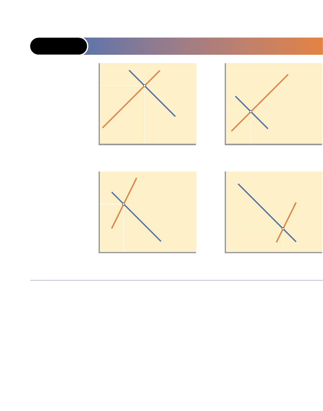
What explains wage differentials such as these? Once again, the forces of demand and

supply are revealing. As we demonstrate in Figure 15-9, wage differentials can arise on

either the supply or demand side of labour markets. Figures 15-9(a) and (b) represent

labour markets for two occupational groups that have identical labour supply curves. The

labour market in panel a has a relatively high equilibrium wage (W

) because labour

demand is very strong. The labour market in panel b has an equilibrium wage that is rel-

atively low (W

) since labour demand is weak. Clearly, the wage differential between

occupations (a) and (b) results solely from differences in the magnitude of labour demand.

Contrast that situation with Figure 15-9(c) and (d), where the labour demand

curves are identical. In the labour market in panel (c), the equilibrium wage is rela-

tively high (W

) because labour supply is highly restricted. In the labour market in

panel (d) labour supply is highly abundant, so the equilibrium wage (W

) is rela-

tively low. The wage differential between (c) and (d) results solely from the differ-

ences in the magnitude of the labour supply.

Although Figure 15-9 provides a good starting point for understanding wage dif-

ferentials, we need to know why demand and supply conditions differ in various

labour markets.

Marginal Revenue Productivity

The strength of labour demand—how far rightward

the labour demand curve is located—differs greatly

among occupations because of differences in how

much various occupational groups contribute to

their employers’ revenue. This revenue contribution,

in turn, depends on the workers’ productivity and

the strength of the demand for the products they are

helping to produce. Where labour is highly produc-

tive and product demand is strong, labour demand

also is strong, and other things equal, pay is high.

Top professional athletes, for example, are highly

productive at sports entertainment, for which mil-

lions of people are willing to pay billions of dollars

over the course of a season. So the marginal revenue

productivity of these top players is exceptionally

high, as are their salaries, represented in Figure

15-9(a). In contrast, in most occupations workers

generate much more modest revenue for their

employers, so their pay is lower, as in Figure 15-9(b).

Noncompeting Groups

On the supply side of the labour market, workers

are not homogeneous; they differ in their mental

chapter ﬁfteen • wage determination, discrimination, and immigration 393

Wage Differentials

wage differ-

entials

The

difference between

the wage received

by one worker or

group of workers

and that received by

another worker or

group of workers.

TABLE 15-3 AVERAGE

WEEKLY WAGES

IN SELECTED

INDUSTRIES, 2000

Average weekly

earnings

(including

Industry overtime)

All industries $ 626.45

Mining, quarrying, and oil wells 1,152.60

Logging and forestry 821.23

Transportation, storage,

communications, and other utilities 779.32

Manufacturing 778.30

Finance, insurance, and real estate 777.52

Construction 722.84

Educational and related services 672.88

Health and social services 542.25

Trade 476.48

Source: Statistics Canada, <www.statcan.ca/english/Pgdb>.

Visit www.mcgrawhill.ca/college/mcconnell9 for data update.

marginal

revenue

productivity

How much workers

contribute to their

employers’ revenue.

and physical capacities and in their education and training. At any given time the

labour force is made up of many noncompeting groups of workers, each repre-

senting several occupations for which the members of a particular group qualify. In

some groups qualiﬁed workers are relatively few, whereas in others they are highly

abundant. Workers in one group do not qualify for the occupations of other groups.

ABILITY

Only a few workers have the ability or physical attributes to be brain surgeons, con-

cert violinists, top fashion models, research scientists, or professional athletes.

Because the supply of these particular types of labour is very small in relation to

labour demand, their wages are high, as in Figure 15-9(c). The members of these and

similar groups do not compete with one another or with other skilled or semiskilled

workers. The violinist does not compete with the surgeon, nor does the surgeon

compete with the violinist or the fashion model.

The concept of noncompeting groups can be applied to various subgroups and

even to speciﬁc individuals in a particular group. An especially skilled violinist can

394 Part Three • Microeconomics of Resource Markets

FIGURE 15-9 LABOUR DEMAND, LABOUR SUPPLY, AND WAGE

DIFFERENTIALS

(a) Strong labour demand

(b) Weak labour demand

(d) Abundant labour supply

The wage differential

between labour

markets (a) and

(b) results solely from

differences in labour

demand. In labour

market (c) and

(d), differences in

labour supply cause

the wage differential.

non-

competing

groups

Collec-

tions of workers in

the economy who

do not compete

with each other

for employment

because the skill

and training of

the workers in one

group are substan-

tially different

from those in other

groups.

command a higher salary than colleagues who play the same instrument. A handful

of top corporate executives earn 10 to 20 times as much as the average chief execu-

tive ofﬁcer. In each of these cases, the supply of top talent is highly limited, since less

talented colleagues are only imperfect substitutes.

EDUCATION AND TRAINING

Another source of wage differentials has to do with differing amounts of investment

in human capital. An investment in human capital is an expenditure on education

or training that improves the skills and, therefore, the productivity of workers. Like expen-

ditures on machinery and equipment, expenditures on education or training that

increase a worker’s productivity can be regarded as investments. In both cases, cur-

rent costs are incurred with the intention that will lead to a greater future ﬂow of

earnings.

Although education yields higher incomes, it carries substantial costs. A college

or university education involves not only direct costs (tuition, fees, books) but indi-

rect or opportunity costs (forgone earnings) as well. Does the higher pay received

by better-educated workers compensate for these costs? The answer is yes. Rates of

return are estimated to be 10 to 13 percent for investments in secondary education

and 8 to 12 percent for investments in college and university education. One gener-

ally accepted estimate is that each year of schooling raises a worker’s wage by about

8 percent. Also, the pay gap between college and university graduates and high-

school graduates increased sharply between 1980 and 2000.

Compensating Differences

If the workers in a particular noncompeting group are equally capable of perform-

ing several different jobs, you might expect the wage rates to be identical for all

these jobs. Not so. A group of high-school graduates may be equally capable of

becoming sales clerks or construction workers, but these jobs pay different wages.

In virtually all locales, construction labourers receive much higher wages than sales

clerks. These wage differentials are called compensating differences, because they

must be paid to compensate for nonmonetary differences in various jobs.

The construction job involves dirty hands, a sore back, the hazard of accidents,

and irregular employment, both seasonally and cyclically. The retail sales job means

clean clothing, pleasant air-conditioned surroundings, and little fear of injury or lay-

off. Other things equal, it is easy to see why some workers would rather pick up a

credit card than a shovel. So labour supply is more limited for construction ﬁrms,

as in Figure 15-9(c), than for retail shops, as in Figure 15-9(d). Construction ﬁrms

must pay higher wages than retailers to compensate for the unattractive nonmone-

tary aspects of construction jobs.

Compensating differences play an important role in allocating society’s scarce

labour resources. If very few workers want to be garbage collectors, then society

must pay high wages to garbage collectors to get the garbage collected. If many

more people want to be sales clerks, then society need not pay them as much as

garbage collectors to get those services performed.

Market Imperfections

The ideas of marginal revenue productivity, noncompeting groups, and differences

in nonmonetary aspects of jobs explain many of the wage differentials in the econ-

omy. But other persistent differentials result from several types of market imperfec-

tions that impede workers from leaving their current jobs to take higher-paying jobs.

chapter ﬁfteen • wage determination, discrimination, and immigration 395

investment

in human

capital

Any

expenditure under-

taken to improve

the education, skills,

health, or mobility

of workers, with

an expectation of

greater productivity

and thus a positive

return on the

investment.

compen-

sating

differences

Differences in the

wages received by

workers in different

jobs to compensate

for nonmonetary

differences in the

jobs.

LACK OF JOB INFORMATION

Workers may simply be unaware of job opportunities and wage rates in other

geographic areas and in other jobs for which they qualify. Consequently, the

ﬂow of qualiﬁed labour from lower-paying to higher-paying jobs—and thus the

adjustments in labour supply—may not be sufﬁcient to equalize wages within

occupations.

GEOGRAPHIC IMMOBILITY

Workers take root geographically. Many are reluctant to move to new places, to

leave friends, relatives, and associates, to force their children to change schools, to

sell their houses, or to incur the costs and inconveniences of adjusting to a new job

and a new community. As Adam Smith noted more than two centuries ago, “A [per-

son] is of all sorts of luggage the most difﬁcult to be transported.” The reluctance or

inability of workers to move creates geographic wage differentials within the same

occupation to persist.

UNIONS AND GOVERNMENT RESTRAINTS

Wage differentials may be reinforced by artiﬁcial restrictions on mobility imposed by

unions and government. We have noted that craft unions ﬁnd it to their advantage

to restrict membership. After all, if carpenters and bricklayers become too plentiful,

the wages they can command will decline. Thus, the low-paid nonunion carpenter

of Edmonton, Alberta, may be willing to move to Vancouver in the pursuit of higher

wages, but her chances for succeeding are slim. She may be unable to get a union

card, and no card means no job. Similarly, an optometrist or lawyer qualiﬁed to prac-

tise in one province may not meet licensing requirements of other provinces, so his

ability to move is limited. Other artiﬁcial barriers involve pension plans and senior-

ity rights that might be jeopardized by moving from one job to another.

DISCRIMINATION

Despite legislation to the contrary, discrimination sometimes results in lower wages

being paid to women and visible-minority workers than to white males doing vir-

tually identical work. Also, women and minorities may be crowded into certain

low-paying occupations, driving down wages there and raising them elsewhere.

If discrimination keeps qualiﬁed women and minorities from taking the higher-

paying jobs, then differences in pay will persist.

All four considerations—differences in marginal revenue productivity, noncom-

peting groups, nonmonetary differences, and market imperfections—come into

play in explaining actual wage differentials. For example, the differential between

the wages of a physician and those of a construction worker can be explained based

on marginal revenue productivity and noncompeting groups. Physicians generate

considerable revenue because of their high productivity and the strong willingness

of consumers (via provincial governments) to pay for health care. Physicians also

fall into a noncompeting group where, because of stringent training requirements,

only a relatively few persons qualify. So the supply of labour is small in relation

to demand.

In some construction work, where training requirements are much less signiﬁ-

cant, the supply of labour is great relative to demand, so, wages are much lower for

construction workers than for physicians. However, if not for the unpleasantness of

the construction worker’s job and the fact that the craft union observes restrictive

membership policies, the differential would be even greater than it is.

396 Part Three • Microeconomics of Resource Markets

The models of wage determination we have described in this chapter assume that

worker pay is always a standard amount for each hour’s work, for example, $15 per

hour. But pay schemes are often more complex than that in both composition and

purpose. For instance, many workers receive annual salaries rather than hourly pay.

Many workers also receive fringe beneﬁts: dental insurance, life insurance, paid

vacations, paid sick-leave days, pension contributions, and so on. Finally, some pay

plans are designed to elicit a desired level of performance from workers. This last

aspect of pay plans requires further elaboration.

The Principal–Agent Problem Revisited

In Chapter 3 we ﬁrst identiﬁed the principal–agent problem as it relates to possible dif-

ferences in the interests of corporate stockholders (principals) and the executives

(agents) they hire. This problem extends to all workers. Firms hire workers because

they are needed to help produce the goods and services the ﬁrms sell for a proﬁt.

Workers are the ﬁrms’ agents; they are hired to advance the interest (proﬁt) of the

ﬁrms. The principals are the ﬁrms; they hire agents to advance their goals. Firms

and workers have one interest in common: they both want the ﬁrm to survive and

thrive. That will ensure proﬁt for the ﬁrm and continued employment and wages for

the workers.

But the interests of the ﬁrm and of the workers are not identical. A principal–

agent problem arises when those interests diverge. Workers may seek to increase

their utility by shirking on the job, that is, by providing less than the agreed-on

effort or by taking unauthorized breaks. They may improve their well-being by

increasing their leisure, during paid work hours, without forfeiting income. The

night security guard in a warehouse may leave work early or spend time reading a

novel rather than making the assigned rounds. A salaried manager may spend time

away from the ofﬁce visiting friends rather than attending to company business.

Firms (principals) have a proﬁt incentive to reduce or eliminate shirking. One

option is to monitor workers, but monitoring is difﬁcult and costly. Hiring another

worker to supervise or monitor the security guard might double the cost of main-

taining a secure warehouse. Another way of resolving the principal–agent problem

is through some sort of incentive pay plan that ties worker compensation more

closely to output or performance. Such incentive pay schemes include piece rates,

commissions and royalties, bonuses and proﬁt sharing, and efﬁciency wages.

PIECE RATES

Piece rates consist of compensation paid according to the number of units of output

a worker produces. If a principal pays fruit pickers by the bushel or typists by the

page, it need not be concerned with shirking or with monitoring costs.

COMMISSIONS OR ROYALTIES

Unlike piece rates, commissions and royalties tie compensation to the value of sales.

Employees who sell products or services—including real estate agents, insurance

agents, stockbrokers, and retail salespersons—commonly receive commissions that

are computed as a percentage of the monetary value of their sales. Recording artists

and authors are paid royalties, computed as a certain percentage of sales revenues

from their works. Such types of compensation link the ﬁnancial interests of the

salespeople or artists and authors to the proﬁt interest of the ﬁrms.

chapter ﬁfteen • wage determination, discrimination, and immigration 397

Pay for Performance

incentive

pay plan

compensation

structure that ties

worker pay directly

to performance

such as piece rates,

bonuses, stock

options, commis-

sions, and proﬁt

sharing.

BONUSES, STOCK OPTIONS, AND PROFIT SHARING

Bonuses are payments in addition to one’s annual salary that are based on some fac-

tor such as the performance of the individual worker, or of a group of workers, or of

the ﬁrm itself. A professional baseball player may receive a bonus based on a high bat-

ting average, the number of home runs hit, or the number of runs batted in. A busi-

ness manager may receive a bonus based on the proﬁtability of her or his unit. Stock

options allow workers to buy shares of their employer’s stock at a ﬁxed, lower price

when the stock price rises. Such options are part of the compensation packages of top

corporate ofﬁcials, as well as many workers in relatively new high technology ﬁrms.

Proﬁt-sharing plans allocate a percentage of a ﬁrm’s proﬁt to its employees. Such plans

have in recent years resulted in large annual payments to many Canadian workers.

EFFICIENCY WAGES

The rationale behind efﬁciency wages is that employers will enjoy greater effort from

their workers by paying them above-equilibrium wage rates. Glance back at Figure

15-3, which shows a competitive labour market in which the equilibrium wage rate

is $10. What if an employer decides to pay an above-equilibrium wage of $12 per

hour? Rather than putting the ﬁrm at a cost disadvantage compared with rival ﬁrms

paying only $10, the higher wage might improve worker effort and productivity so

that unit labour costs actually fall. For example, if each worker produces 10 units of

output per hour at the $12 wage rate compared with only 6 units at the $10 wage

rate, unit labour costs for the high-wage ﬁrm will be only $1.20 (= $12 ÷ 10) com-

pared to $1.67 (= $10 ÷ 6) for ﬁrms paying the equilibrium wage.

An above-equilibrium wage may enhance worker efﬁciency in several ways. It

enables the ﬁrm to attract higher-quality workers, it lifts worker morale, and it low-

ers turnover, resulting in a more experienced workforce, greater worker productiv-

ity, and lower recruitment and training costs. Because the opportunity cost of losing

a higher-wage job is greater, workers are more likely to put forth their best efforts

with less supervision and monitoring. In fact, efﬁciency wage payments have

proven effective for many employers.

Addenda: The Negative Side Effects of Pay for Performance

Although pay for performance may help to overcome the principal–agent problem

and enhance worker productivity, such plans may have negative side effects and so

require careful design. Here are a few examples:

● The rapid production pace that piece rates encourage may result in poor prod-

uct quality and may compromise the safety of workers. Such outcomes can be

costly to the ﬁrm over the long run.

● Commissions may cause some salespeople to engage in questionable or even

fraudulent sales practices, such as making exaggerated claims about products

or recommending unneeded repairs. Such practices may lead to private law-

suits or government legal action.

● Bonuses based on personal performance may disrupt the close cooperation

needed for maximum team production. A professional basketball player who

receives a bonus for points scored may be reluctant to pass the ball to teammates.

● Since proﬁt sharing is usually tied to the performance of the entire ﬁrm, less

energetic workers can free-ride by obtaining their proﬁt share based on the

hard work of others.

398 Part Three • Microeconomics of Resource Markets

● There may be a downside to the reduced turnover resulting from above-market

wages: Firms that pay efﬁciency wages have fewer opportunities to hire new

workers and suffer the loss of new blood that sometimes energizes the workplace.

Broadly deﬁned, labour market discrimination occurs when equivalent labour

resources are paid or treated differently even though their productive contributions

are equal. These differences result from a combination of nondiscriminatory and

discriminatory factors. For example, studies indicate that about one-half the differ-

ences in earnings between men and women and between whites and visible minori-

ties can be explained by such nondiscriminatory factors as differences in education,

age, training, industry and occupation, union membership, location, work experi-

ence, continuity of work, and health. (Of course, some of these factors may be inﬂu-

enced by discrimination.) The other half is an unexplained difference, the bulk of

which economists attribute to discrimination

In labour market discrimination, certain groups of people are often accorded infe-

rior treatment with respect to hiring, occupational access, education and training,

promotion, wage rates, or working conditions even though they have the same abil-

ities, education and training, and experience as the more preferred groups. People

who practise discrimination are said to exhibit a prejudice or bias against the targets

of their discrimination.

Types of Discrimination

Labour market discrimination may take several forms:

● Wage discrimination occurs when women or members of minorities are paid

less than white males for doing the same work. This kind of discrimination is

declining because of its explicitness and the fact that it clearly violates federal

law. But wage discrimination can be subtle and difﬁcult to detect. For exam-

ple, women and minorities sometimes ﬁnd that their job classiﬁcations carry

lower pay than job classiﬁcations held by white males, even though they are

performing essentially the same tasks.

chapter ﬁfteen • wage determination, discrimination, and immigration 399

Labour Market Discrimination

<is.dal.ca/~eequity/

INFO/question.htm>

Frequently asked

employment equity

questions

● Proponents of the minimum wage argue that it

is needed to assist the working poor and to

counter monopsony where it might exist; critics

say that it is poorly targeted to reduce poverty

and that it reduces employment.

● Wage differentials are generally attributable to

the forces of supply and demand, inﬂuenced by

differences in workers’ marginal revenue pro-

ductivity, workers’ education and skills, and non-

monetary differences in jobs. Several labour

market imperfections also play a role.

● As it applies to labour, the principal–agent prob-

lem is one of workers pursuing their own inter-

ests to the detriment of the employer’s proﬁt

objective.

● Pay-for-performance plans (piece rates, com-

missions, royalties, bonuses, proﬁt sharing, and

efficiency wages) are designed to improve

worker productivity by overcoming the principal–

agent problem.

wage dis-

crimination

The payment of a

lower wage to

members of a less-

preferred group

than to members of

a more-preferred

group for the same

work.

● Employment discrimination takes place when women or visible-minority

workers receive inferior treatment in hiring, promotions, assignments, tem-

porary layoffs, and permanent discharges. This type of discrimination also

encompasses sexual and racial harassment—demeaning treatment in the

workplace by coworkers or administrators.

● Occupational discrimination occurs when women or visible-minority work-

ers are arbitrarily restricted or prohibited from entering the more desirable,

higher-paying occupations. Businesswomen have found it difﬁcult to break

through the “glass ceiling” that prevents them from moving up to executive

ranks. Visible minorities in executive and sales positions are relatively rare. In

addition, skilled and unionized work such as electrical work, bricklaying, and

plumbing do not have high visible minority representation.

● Human capital discrimination occurs when women or members of minorities

do not have the same access to productivity-enhancing investments in education

and training as white males. For example, the lower average educational attain-

ment of visible minorities has reduced their opportunities in the labour market.

Costs of Discrimination

Discrimination imposes costs on those who are discriminated against. The groups

that discriminate get the good jobs and the better pay that are withheld from the tar-

gets of discrimination. But discrimination does more than simply transfer beneﬁts

from women and visible minorities to men and whites; where it exists, discrimina-

tion actually diminishes the economy’s output and income; like any other artiﬁcial

barrier to free competition, it decreases economic efﬁciency and reduces production.

By arbitrarily blocking certain qualiﬁed groups of people from high-productivity

(and thus high-wage) jobs, discrimination prevents them from making their maxi-

mum contribution to society’s output, income, and well-being.

The effects of discrimination can be depicted as a point inside the economy’s pro-

duction possibilities curve, such as point D in Figure 15-10. At such a point, the econ-

omy obtains some combination of capital and consumption goods—here, K

—that is less desirable than combinations represented by points such as X, Y, or Z

on the curve. By preventing the economy from achieving productive efﬁciency, dis-

crimination reduces the nation’s real output and income. Very rough estimates suggest

that the Canadian economy would gain $32 billion per year by eliminating racial and

ethnic discrimination and some $18 billion per year by ending gender discrimination.

Prejudice reﬂects complex, multifaceted, and deeply ingrained beliefs and atti-

tudes. Thus, economics can contribute some insight into discrimination but no

detailed explanations. With this caution in mind, let’s look more deeply into the eco-

nomics of discrimination.

Taste-for-Discrimination Model

The taste-for-discrimination model examines prejudice by using the emotion-free

language of demand theory. It views discrimination as resulting from a preference

or taste for which the discriminator is willing to pay. The model assumes that, for

whatever reason, prejudiced people experience a subjective or psychic cost—a

400 Part Three • Microeconomics of Resource Markets

employment

discrimina-

tion

Inferior

treatment in hiring,

promotion, and

work assignment

for a particular

group of employees.

occupa-

tional dis-

crimination

Arbitrary restriction

of particular groups

from more desir-

able, higher-paying

occupations.

human

capital

discrimina-

tion

Arbitrary

restriction of par-

ticular groups

from productivity-

enhancing invest-

ments in education

and training.

Economic Analysis of Discrimination

taste-for-

discrimina-

tion model

theory of discrimi-

nation that views it

as a preference for

which an employer

is willing to pay.