Middleton W.M. (ed.) Reference Data for Engineers: Radio, Electronics, Computer and Communications
Подождите немного. Документ загружается.

32-48
REFERENCE
DATA
FOR ENGINEERS
The sidelobe ratio is given by
SLR
=
20 log
(sinh
rB/
rB)
+
13.26 dB
Taking the inverse transform of the pattern gives the
Taylor one-parameter line source distribution:
where
p
is
0
at the aperture center and
1
at each end,
I,
is the modified Bessel function.
A special case occurs for
B
=
0.
This is the uni-
formly excited line source (constant amplitude), which
has a pattern of simply sin
m/m.
The Taylor pattern
is a modified sin
m/m
pattern, with a transition from
that to the hyperbolic form at
u
=
B,
on the side of the
main beam. The hyperbolic form provides the central
part of the main beam as indicated in the formula
above for
SLR.
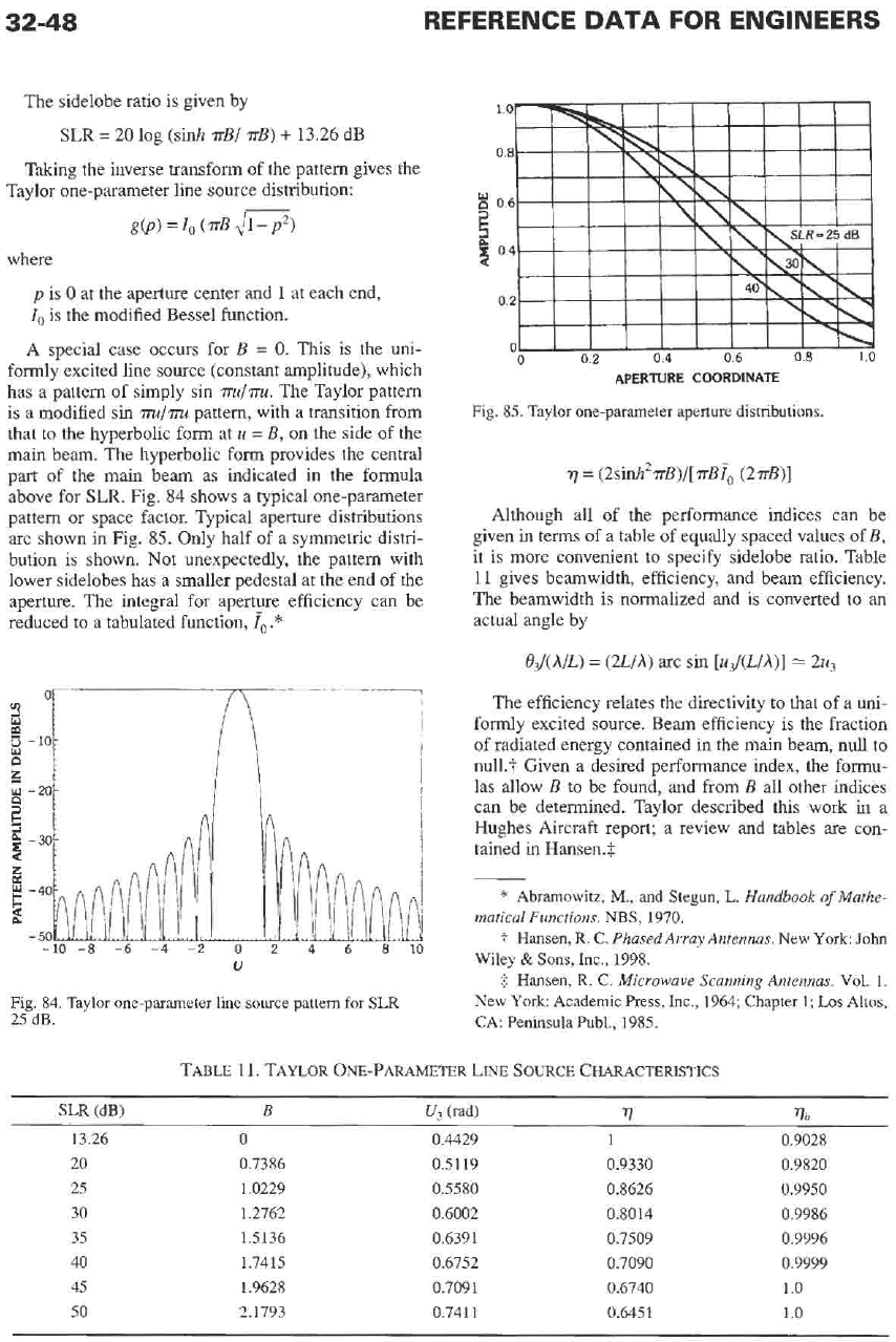
Fig.
84
shows a typical one-parameter
pattern or space factor. Typical aperture distributions
are shown in Fig.
85.
Only half of a symmetric distri-
bution is shown. Not unexpectedly, the pattern with
lower sidelobes has a smaller pedestal at the end of the
aperture. The integral for aperture efficiency can be
reduced to
a
tabulated function,
f,
.*
ii
J
-10
"/
w
a
U
Fig.
84.
Taylor one-parameter line source pattern for
SLR
25
dB.
0.2
0
0
0.2
0.4
0.6 0.8
1.0
APERTURE COORDINATE
Fig.
8.5.
Taylor one-parameter aperture distributions.
77
=
(2siwt2~~)/[r~fO
(2~~11
Although all
of
the performance indices can be
given
in
terms of a table of equally spaced values of
B,
it is more convenient
to
specify sidelobe ratio. Table
11
gives beamwidth, efficiency, and beam efficiency.
The beamwidth is normalized and is converted
to
an
actual angle by
B,/(A/L)
=
(2L/A) arc sin
[u,/(L/A)]
2u,
The efficiency relates the directivity to that of a uni-
formly excited source. Beam efficiency is the fraction
of radiated energy contained in the main beam,
null
to
null.? Given a desired performance index, the formu-
las allow
B
to
be found, and from
B
all other indices
can be determined. Taylor described this work in a
Hughes Aircraft report; a review and tables are con-
tained in Hamen.$
*
Abrarnowitz,
M.,
and Stegun,
L.
Handbook
of
Mathe-
matical Functions. NBS,
1970.
t
Hansen,
R.
C.
PhasedArray Antennas.
New
York:
John
Wiley
&
Sons,
Inc.,
1998.
$
Hansen,
R.
C.
Microwave Scanning Antennas.
Vol.
1.
New
York: Academic
Press,
Inc.,
1964;
Chapter
1;
Los
Altos,
CA: Peninsula Publ.,
198.5.
TABLE
11.
TAYLOR ONE-PARAMETER LINE SOURCE CHARACTERISTICS
U3
(rad)
77
776
SLR
(dB)
B
13.26
0
0.4429 1 0.9028
20
25
30
3.5
40
45
50
0.7386
1.0229
1.2762
1.5136
1.7415
1.9628
2.1793
0.5119 0.9330 0.9820
0.5.580 0.8626 0.9950
0.6002 0.8014 0.9986
0.6391 0.7.509 0.9996
0.6752 0.7090 0.9999
0.7091 0.6740
1
.o
0.7411 0.6451 1
.o
ANTENNAS
32-49
Taylor
ii
Line Source
Distribution
A modest improvement in efficiency can be
obtained by making the first few sidelobes at equal
level, with a transition from the equal-level envelope to
the
l/u
envelope. This offers a compromise between
the one-parameter distribution and the Chebyshev dis-
tribution.
In
the latter, the sidelobes are all of equal
height, the aperture distribution is singular at the ends,
the energy storage is high, and the distribution is sensi-
tive to errors. For
E
small, the distribution gives
improved efficiency and narrower beamwidth without
significantly degrading its robust nature. The distribu-
tion is a modification of the continuous equivalent of a
Chebyshev distribution, with a dilation factor used to
modify the first
Z
zeros. The pattern is given by a
canonical product on zeros.*
n=l
n=&l
=
zF(n,A,
n)sinc
T(U
+
n)
n=-(E-i)
In
the second form, the pattern
is
a superposition of
E
sinc beams. The pattern coefficients are
2
[(Ti
-
l)!]
(E
-
1
+
a)!(
n
-
1
-
n)!
F(n,A,Ti)
=
with
F(0,
A,
E)
=
1.
Here the zeros are:
Z,=f(~,/A~+(n-1/2)~ 15nS
7i
Zn=irn
E4n
where
A
is the sidelobe parameter,
(T
is the dilation index.
The dilation index is
(T
=Ti/JW
The corresponding aperture distribution is
E-1
g(p)=1+2zF(n,A,E)cosnnp
n=l
Tables of aperture distribution are not given because
of the ease of calculating these with a computer. Val-
ues for check purposes can be obtained from Hansen.?
Table
12
gives parameter
A
and beamwidth factor
u3
for several values
of
SLR.
Also shown are
(T
values for
E.
The beamwidth in
u
is approximately
2m,;
this
may be converted
to
angle by using the formula in the
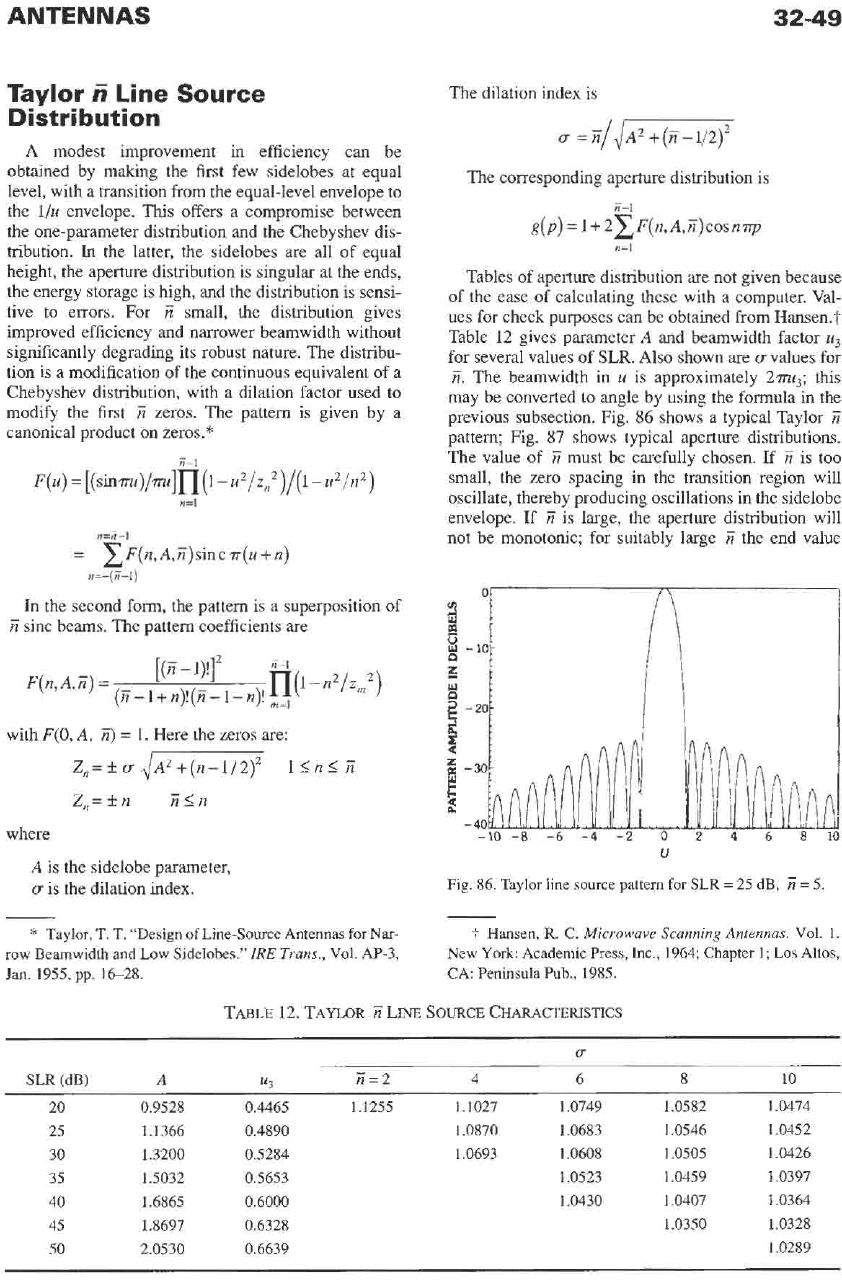
previous subsection. Fig.
86
shows a typical Taylor
Ti
pattern; Fig.
87
shows typical aperture distributions.
The value of
E
must be carefully chosen. If
ii
is too
small, the zero spacing
in
the transition region will
oscillate, thereby producing oscillations in the sidelobe
envelope. If
7i
is large, the aperture distribution will
not be monotonic; for suitably large
E
the end value
10
w
n
5
-20
$
z
i!
-30
E
-
40
-10
-8 -6
-4
-2
0
2
4
6 8
1’
u
Fig.
86.
Taylor
line source
pattern for
SLR
=
25
dB,
E
=
5.
*
Taylor,
T.
T.
“Design
of
Line-Source
Antennas
for
Nar-
row
Beamwidth
and
Low
Sidelobes.”
IRE
Trans.,
Vol.
AP-3,
.Jan.
1955,
pp.
16-28.
t
Hansen,
R.
C.
Microwave Scanning Antennas.
Vol.
1.
New
York:
Academic Press, Inc.,
1964;
Chapter
1;
Los
Altos,
CA:
Peninsula Pub.,
1985.
TABLE
12.
TAYLOR
E
LINE
SOURCE CHARACTERISTICS
U
SLR
(dB)
A
u3
n=2 4 6 8 10
20 0.9528 0.4465 1.1255 1.1027 1.0749 1.0582 1.0474
25 1.1366 0.4890 1.0870 1.0683 1.0546 1.0452
30
1.3200 0.5284 1.0693 1.0608 1.0505 1.0426
35 1.5032 0.5653 1.0523 1.0459 1.0397
40 1.6865 0.6000 1.0430 1.0407 1.0364
45 1.8697 0.6328 1.0350 1.0328
50
2.0530 0.6639 1.0289
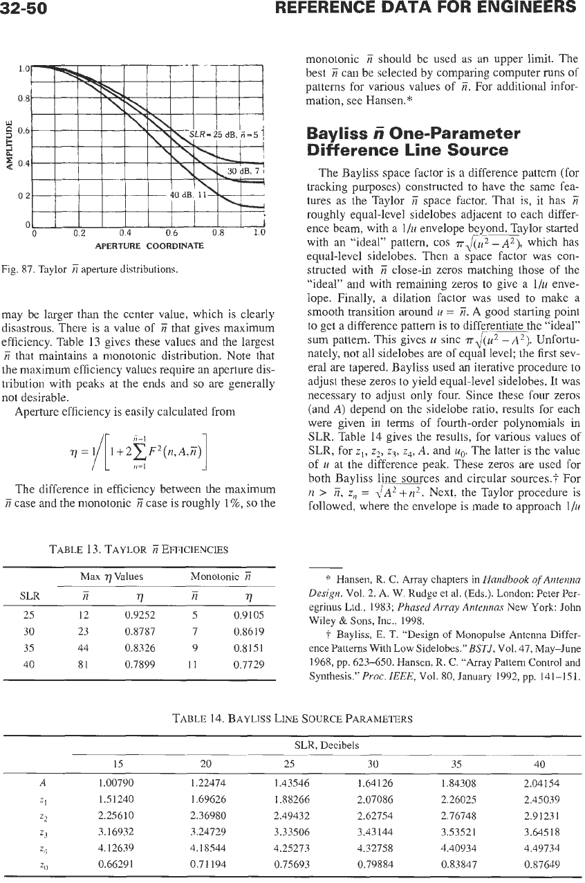
32-50
REFERENCE
DATA
FOR ENGINEERS
10
08
w
0
06
2
2
3
04
02
0
0
02
04
06
08
10
APERTURE COORDINATE
Fig.
87.
Taylor
E
aperture distributions.
may be larger than the center value, which is clearly
disastrous. There is a value of
E
that gives maximum
efficiency. Table
13
gives these values and the largest
E
that maintains a monotonic distribution. Note that
the maximum efficiency values require an aperture dis-
tribution with peaks at the ends and
so
are generally
not desirable.
Aperture efficiency is easily calculated from
1
ii-1
17
=
1
1+2xF2(n,A,E)
/[
n=l
The difference
in
efficiency between the maximum
E
case and the monotonic
Ti
case is roughly
1%,
so
the
TABLE
13.
TAYLOR
E
EFFICIENCIES
Max
17
Values Monotonic
Ti
-
-
SLR
Iz
r)
n
rl
25 12
0.9252
5
0.9105
30 23
0.8787 7 0.8619
35 44 0.8326 9 0.8151
40 81
0.7899 11 0.7729
monotonic
Ti
should be used as
an
upper limit. The
best
E
can be selected by comparing computer
runs
of
patterns for various values of
Z.
For additional infor-
mation, see Hansen.*
Bayliss
E
One-Parameter
Difference Line Source
The Bayliss space factor is a difference pattern (for
tracking purposes) constructed to have the same fea-
tures as the Taylor
E
space factor. That
is,
it has
Ti
roughly equal-level sidelobes adjacent to each differ-
ence beam, with a
1/u
envelope beyond. Taylor started
with
an
“ideal” pattern, cos
TJ-,
which has
equal-level sidelobes. Then a space factor was con-
structed with
E
close-in zeros matching those of the
“ideal” and with remaining zeros to give a
l/u
enve-
lope. Finally, a dilation factor was used to make a
smooth transition around
u
=
E.
A
good starting point
to
get a difference pattern is
to
differentiate the “ideal”
sum pattern.
hi^
gives
u
sinc
n-&Uz_A2).
Unfortu-
nately, not all sidelobes are of equal level; the first sev-
eral
are
tapered. Bayliss used an iterative procedure to
adjust these zeros to yield equal-level sidelobes. It was
necessary to adjust only four. Since these four zeros
(and
A)
depend on the sidelobe ratio, results for each
were given
in
terms
of
fourth-order polynomials
in
SLR.
Table
14
gives the results, for various values of
SLR,
for
zl,
z2,
z3,
z4,
A.
and
uO.
The latter is the value
of
u
at the difference peak. These zeros are used for
both Bayliss line sources and circular sources.? For
n
>
E,
z,%
=
%m.
Next, the Taylor procedure is
followed, where the envelope is made to approach
l/u
*
Hansen, R.
C.
Array chapters in
Handbook
of
Antenna
Design.
Vol.
2.
A.
W. Rudge et
al.
(Eds.).
London: Peter Per-
egrinus Ltd.,
1983;
Phased Array Antennas
New York:
John
Wiley
&
Sons,
Inc.,
1998.
7
Bayliss,
E.
T. “Design of
Monopulse
Antenna Differ-
ence Patterns With Low Sidelobes.”BSTJ, Vol.
47,
May-June
1968,
pp.
623-650.
Hansen, R. C. “Array Pattern
Control
and
Synthesis.”
Proc.
ZEEE,
Vol.
80,
January
1992,
pp.
141-151.
TABLE
14.
BAYLISS LINE SOURCE PARAMETERS
SLR, Decibels
15 20 25 30 35 40
A
1.00790
1.22474 1.43546
1.64126 1.84308
2.04154
-71
1.5 1240
1.69626 1.88266
2.07086 2.26025 2.45039
z2
2.25610
2.36980 2.49432
2.62754 2.76748 2.91231
z3
3.16932 3.24729 3.33506
3.43 144
3.53521 3.645 18
z4
4.12639
4.18544 4.25273
4.32758
4.40934 4.49734
20
0.66291 0.71194 0.75693 0.79884 0.83847 0.87649
ANTENNAS
32-5
1
for large
u,
and with a smooth transition. The differ-
ence pattern is
E-1
IS-
(1
-
u”cT
2zn2)
n(1-
u2/(n+
1/2)2)
F(u)
=
ucosm
=
,-;=I
n=o
As before,
a=(?i+
1/2)/\/A2+E2
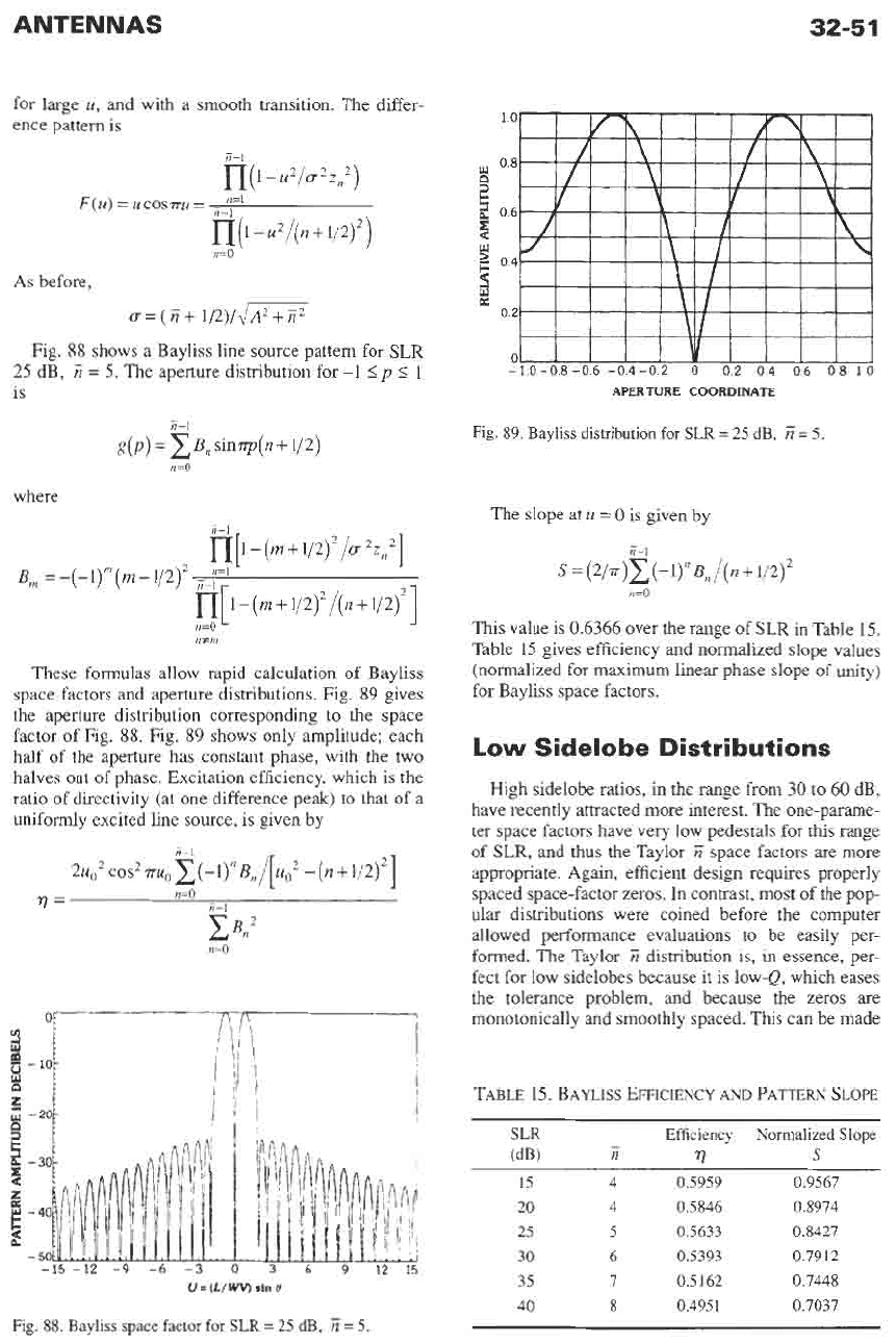
Fig.
88
shows a Bayliss line source pattern for SLR
25 dB,
ti
=
5.
The aperture distribution for
-1
5
p
5
1
is
ii-1
g(P)
=
CB.
sinnp(
n+
1/2)
n=O
where
E-1
n[l-
(m
+
1/2)2/a
24
’I
n[
1
-
(rn
+
1/2)2/(n
+
1/2)
B,
=
-(-1)m(m-1/2)2
&;=I
n=O
ntm
These formulas allow rapid calculation of Bayliss
space factors and aperture distributions. Fig.
89
gives
the aperture distribution corresponding to the space
factor of Fig.
88.
Fig.
89
shows only amplitude; each
half
of
the aperture has constant phase, with the two
halves out of phase. Excitation efficiency, which is the
ratio of directivity (at one difference peak) to that of a
uniformly excited line source, is given by
E-1
2u02 Cos2mo~(-l)nBn/[uo~ -(n+1/2)2]
n=O
77=
E-l
CBn2
n=O
8
-I0
X
CI
$
-30
z
E
-40
-
50
;
-20
a
i
L
-15
-12
-9
-6
-3
0
3
6
9
12
15
1.0
0.8
D
5
0.6
F
a
w
E
0.4
CT
0.2
0
-1.0-0.8-0.6-0.4-0.2
0
0.2
0.4
0.6
0.8
1.0
APERTURE
COORDINATE
Fig.
89.
Bayliss distribution for
SLR
=
25
dB,
E
=
5.
The slope at
u
=
0
is given by
ii-1
s
=
(2/T)C(-l)nB,,/(n+1/2)2
FO
This value is
0.6366
over the range of SLR in Table 15.
Table 15 gives efficiency and normalized slope values
(normalized for maximum linear phase slope of unity)
for Bayliss space factors.
Low
Sidelobe
Distributions
High sidelobe ratios, in the range from
30
to
60
dB,
have recently attracted more interest. The one-parame-
ter space factors have very low pedestals for this range
of SLR, and
thus
the Taylor
E
space factors are more
appropriate. Again, efficient design requires properly
spaced space-factor zeros. In contrast, most of the pop-
ular distributions were coined before the computer
allowed performance evaluations to be easily per-
formed. The Taylor
E
distribution is, in essence, per-
fect for low sidelobes because it is low-Q, which eases
the tolerance problem, and because the zeros are
monotonically and smoothly spaced. This can be made
TABLE 15. BAYLISS EFFICIENCY
AND
PATTERN SLOPE
Efficiency Normalized Slope
-
(dB)
n
77
S
SLR
15 4
0.5959 0.9567
20 4 0.5846
0.8974
25 5 0.5633 0.8427
30
6 0.5393 0.7912
35 7
OS162 0.7448
40
8
0.495
1
0.7037
Fig.
88.
Bayliss space factor for
SLR
=
25
dB,
E
=
5.
32-52
REFERENCE
DATA
FOR ENGINEERS
evident by comparing the Taylor with the popular
Hamming distribution. The latter* is
g(p)
=
0.54
+
0.46 cos
np
=
a
+
b
cos
np
The excitation efficiency of the Hamming is
=
2a2/(2a2
+
b2)
=
0.7338
The space factor has zeros at
u
=
2,
3, 4
....
and, in
addition, a zero at
u
= =
2.5981.
This close
spacing of the first three zeros produces an uneven
sidelobe envelope with the fourth sidelobe the highest
at 42.7 dB. Thus, the Hamming is compared with a
Taylor
E
distribution with
SLR
=
42.7 dB. Table 16
shows the zeros, and it can be observed that both
of
the
Taylor space factors have a smoothly increasing zero
spacing from the first zero out to the transition point,
beyond which the spacing is unity. The Hamming, on
the other hand, has a first spacing of
0.598,
a second
spacing
of
0.402, and the remaining spacings all unity.
This is obviously not
as
good a design, as the follow-
ing will show.
Table 17 gives efficiency and normalized beam-
width for the three Taylor cases and for the Hamming.
It may be seen that the Hamming beamwidth is
TABLE 16.
ZEROS OF DISTRIBUTIONS
FOR
SLR
=
42.7
DB
Taylor
n
One-Parameter Taylor Hamming
E=6 E=lO
1
2
3
4
5
6
7
8
9
10
2.112
2.732
3.550
4.412
5.335
6.282
7.243
8.214
9.190
10.172
1.894 1.897
2.398 2.396
3.173 3.166
4.069 4.056
5.020 5.002
6 5.978
7 6.970
8
7.974
9 8.984
10
10
2
2.598
3
4
5
6
7
8
9
10
TABLE 17. COMPARISON
OF
DISTRIBUTIONS
FOR
SLR
=
42.7
DB
Taylor
One-Parameter Taylor Hamming
E=6 E=lO
roughly 3% broader, while the efficiency is roughly
3% lower. Thus, by use of appropriate space factors
such as the Taylor
E,
improved performance can be
obtained at no additional cost in complexity, hardware,
or tolerances. For rectangular arrays with separable
aperture distributions, Taylor distributions may, of
course, be used along each coordinate. For circular
disk apertures, the circular Taylor
E
distribution is
similarly excellent.
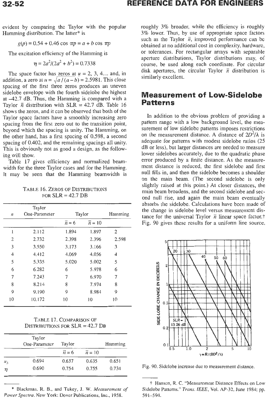
Measurement
of
Low-Sidelobe
Patterns
In
addition to the obvious problem of providing a
pattern range with a low background level, the mea-
surement
of
low sidelobe patterns imposes restrictions
on the measurement distance. A distance of
W2/h
is
adequate for patterns with modest sidelobe ratios (25
dB
or less), but larger distances are needed
to
measure
lower sidelobes accurately, due to the quadratic phase
error produced by a finite distance.
As
the measure-
ment distance is reduced, the first sidelobe and first
null fills in, and then the sidelobe becomes a shoulder
on the main beam. (The second sidelobe is only
slightly raised at this point.) At closer distances, the
main beam broadens, and the second sidelobe and sec-
ond null rise, and again the main beam eventually
absorbs the sidelobe. Calculations have been made of
the change in sidelobe level versus measurement dis-
tance for the universal Taylor
E
linear space factor.?
Fig.
90
gives these results for a uniform line source,
u
z
x
E
00
il
P
s
%
0
0
0.5
1.0
2
5
10
Y
=R/(2@/!4
u3
0.694
0.637 0.635
0.651
rl
0.690
0.754
0.755 0.734
Fig.
90.
Sidelobe increase due to measurement distance.
*
Blackman,
R.
B.,
and Tukey,
J.
W.
Measurement
of
Power Spectra.
New
York: Dover Publications,
Inc.,
1958.
f
Hansen,
R.
C.
“Measurement Distance Effects on
Low
Sidelobe Patterns.”
Trans.
IEEE,
Vol.
A€-32,
June
1984;
pp.
591-594.
ANTENNAS
32-53
and for
20
(10)
60-dB Taylor
Ti
line sources. Distance
is normalized to
2D2/A,
where
y
=
R/(2D2/A)
Each curve terminates when the sidelobe becomes a
shoulder on the main beam, without any dip.
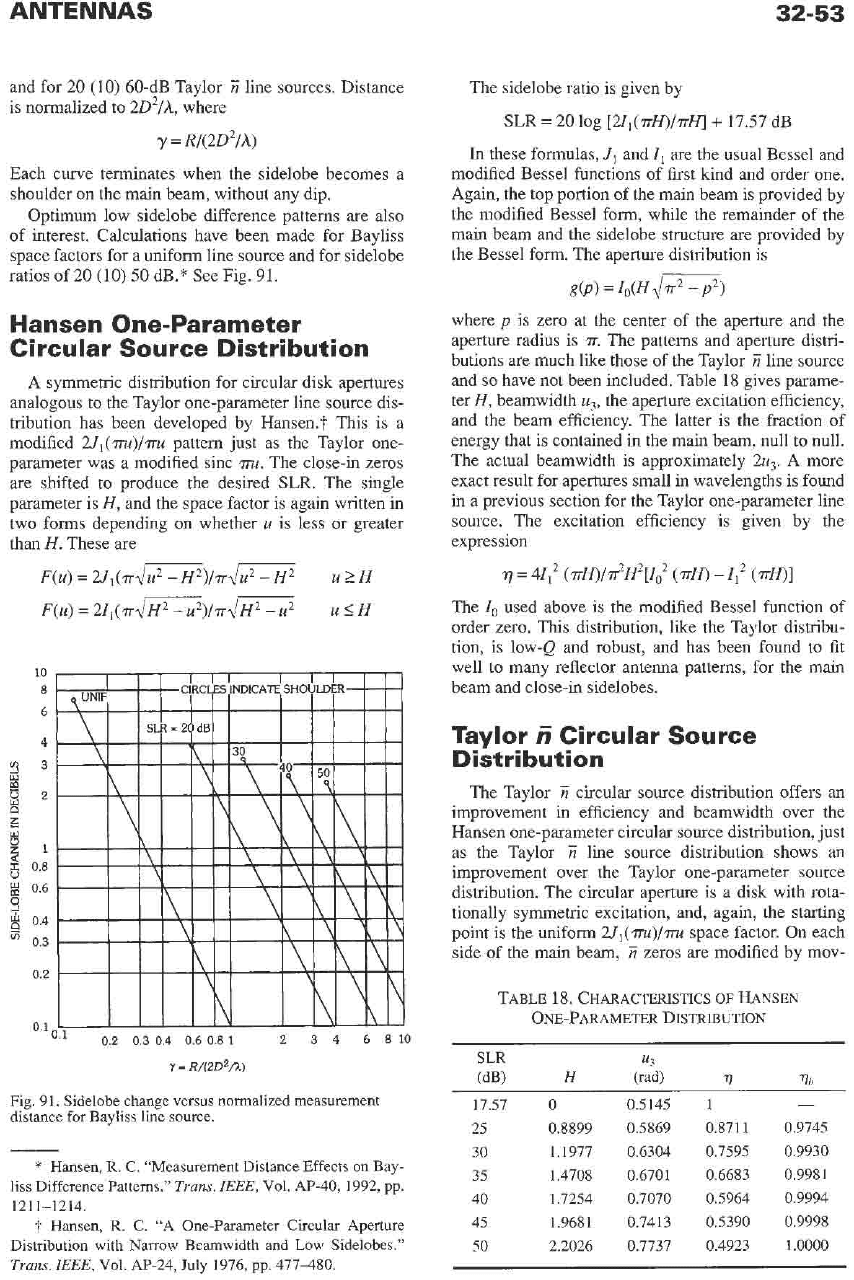
Optimum low sidelobe difference patterns are also
of interest. Calculations have been made for Bayliss
space factors for a uniform line source and for sidelobe
ratios of
20
(10)
50
dB.* See Fig.
91.
Hansen One-Parameter
Circular Source Distribution
A
symmetric distribution for circular disk apertures
analogous to the Taylor one-parameter line source dis-
tribution has been developed by Hansen.t This is a
modified
Ul(m)/m
pattern
just
as the Taylor one-
parameter was a modified sinc
m.
The close-in zeros
are shifted to produce the desired
SLR.
The single
parameter is
H,
and the space factor is again written in
two forms depending on whether
u
is less or greater
than
H.
These are
F(u)
=
Ul(n~m)/r~m
F(u)
=
211(rrJFi2-U2)/~JH2
-u2
u
2
H
u
I
H
Y
=
R/(2D2/;1)
Fig.
91.
Sidelobe change versus normalized measurement
distance for Bayliss
line
source.
*
Hansen,
R.
C. “Measurement Distance Effects
on
Bay-
liss
Difference Patterns.”
Trans.
IEEE,
Vol.
AP-40, 1992,
pp.
1211-1214.
t
Hansen,
R.
C. “A One-Parameter Circular Aperture
Distribution with
Narrow
Beamwidth and Low Sidelobes.”
Trans.
IEEE,
Vol.
Ap-24,
July
1976,
pp.
477480.
The sidelobe ratio is given by
SLR
=
20
log
[2I,(mH)/rfl
+
17.57
dB
In
these formulas,
J1
and
I,
are the usual Bessel and
modified Bessel functions of first kind and order one.
Again, the top portion of the main beam is provided by
the modified Bessel form, while the remainder of the
main beam and the sidelobe structure
are
provided by
the Bessel form. The aperture distribution is
g(P)
=
Io(HJ~)
where
p
is zero at the center
of
the aperture and the
aperture radius is
T.
The patterns and aperture distri-
butions are much like those of the Taylor
E
line source
and
so
have not been included. Table
18
gives parame-
ter
H,
beamwidth
uj,
the aperture excitation efficiency,
and the beam efficiency. The latter is the fraction of
energy that is contained in the main beam, null to null.
The actual beamwidth is approximately
2u,.
A more
exact result for apertures small in wavelengths is found
in a previous section for the Taylor one-parameter line
source. The excitation efficiency
is
given by the
expression
7
=
41,’
(
TH)/dH2[I;
(
TH)
-
1,’
(
TH)]
The
Io
used above is the modified Bessel function of
order zero. This distribution, like the Taylor distribu-
tion, is low-Q and robust, and has been found
to
fit
well to many reflector antenna patterns, for the main
beam and close-in sidelobes.
Taylor
i
Circular Source
Distribution
The Taylor
?i
circular source distribution offers an
improvement in efficiency and beamwidth over the
Hansen one-parameter circular source distribution, just
as the Taylor
ii
line source distribution shows
an
improvement over the Taylor one-parameter source
distribution. The circular aperture is a disk with rota-
tionally symmetric excitation, and, again, the starting
point is the uniform
2J1(m)/m
space factor. On each
side of the main beam,
E
zeros are modified by mov-
TABLE
18.
CHARACTERISTICS
OF
HANSEN
ONE-PARAMETER
DISTRI~UTTON
SLR
(dB)
17.57
25
30
35
40
45
50
u3
H
(rad)
77
96
0 0.5145
1
-
0.8899
0.5869 0.8711
0.9745
1.1977 0.6304
0.7595 0.9930
1.4708 0.6701
0.6683 0.9981
1.7254
0.7070 0.5964
0.9994
1.9681 0.7413
0.5390 0.9998
2.2026
0.7737 0.4923
1.0000
32-54
REFERENCE
DATA
FOR ENGINEERS
ing them to produce the desired sidelobe ratio.* Again,
a dilation factor,
a,
is used to provide a smooth transi-
tion between the roughly equal-level sidelobes and the
tapered-envelope sidelobes. The pattern is given by a
canonical product on zeros:
where
pn
are
the zeros of
J,(m).
The close-in pattern
zeros
are
given by
u,=+~~A~+(n-1/2)~ 15nS
E
while
u
=pE
dA2+(E-1/2)2
Table
19
gives the sidelobe parameter,
A,
the beam-
width,
ug,
and values of
a
for various values of
E.
The
actual beamwidth for large apertures is
2a,.
The pat-
terns and aperture distributions are much like those
of
the Taylor
E
line source and
so
have not been
included. The aperture distribution is
where
p
=
2.rrp/D
*
Taylor,
T. T.
“Design of Circular Apertures for Narrow
Beamwidths and Low Sidelobes.”
IRE
Trans,
AP-8, 1960
pp.
17-22.
and
All of these formulas
are
easily computed,
so
no
tables have been included. For checking purposes, ref-
erence may be made to tables
of
Hansen.? The aper-
ture excitation efficiency is given by
Table
20
gives the aperture excitation efficiency for
several combinations of SLR and
E.
REFLECTORS
Parabolic Reflectors
The parabolic reflector commonly exists in both
focal feed and Cassegrain form (Figs.
92
and
93).
Off-
set reflectors are covered later. For a front-fed reflector,
the reflector
flD
must be matched to the feed pattern.
Reflectors with pattern sidelobes roughly
-25
dB and
t
Hansen,
R.
C. “Tables
of
Taylor Distributions for
Cir-
cular Aperture Antennas.”
IRE
Trans.,
Vol.
AP-8,
January
1960,
pp.
23-26.
Hansen,
R.
C.
Phased Array Antennas.
New
York
John
Wiley
&
Sons,
Inc.,
1998.
TABLE
19.
TAYLOR CIRCULAR SOURCE CHARACTERISTICS
rl
SLR
(a)
A
u3
n=4 5 6 7 8 9 10
20 0.9528 0.4465
1.1692 1.1398 1.1186 1.1028 1.0906 1.0810 1.0732
25 1.1366 0.4890
1.1525 1.1296 1.1118 1.0979 1.0870 1.0782 1.0708
30 1.3200 0.5284 1.1338 1.1180 1.1039 1.0923 1.0827
1.0749 1.0683
35 1.5032 0.5653
1.1134 1.1050
1.0951 1.0859 1.0779 1.0711 1.0653
40 1.6865 0.6000 1.0916 1.0910 1.0854 1.0789 1.0726 1.0670 1.0620
TABLE
20.
EXCITATION EFFICIENCY
VERSUS
E
7
SLR
(a)
n=4 5 6
8
10
20 0.9723 0.9356 0.8808 0.7506 0.6238
25 0.9324 0.9404 0.9379 0.9064 0.8526
30 0.8482 0.8623 0.8735 0.8838 0.8804
35 0.7708 0.7779 0.7880 0.8048 0.8153
40
0.7056 0.7063 0.71 19 0.7252 0.7365
ANTENNAS
32-55
-u
y
=
2f
tan
(8/2)
Fig.
92.
Paraboloidal-reflector design.
PARABOLOIDAL
HYPERBOLOIDAL
Effective
focal
length
f,-
Ir,/fb)fc
Fig.
93.
Cassegrain reflector system.
good efficiency typically have illumination edge tapers
of
-
10
to
-
1
1dB. For lower sidelobes, the edge taper
must be lower. The tradeoff between edge taper and
sidelobe level can be accurately determined from the
circular one-parameter distributions in
the
section on
aperture distributions. Fig. 94 shows the total reflector
subtended angle versusflD, where
0
=
2
arc tan
[(SflD)/(16f2/D2
-
l)]
Fig. 95 gives the differential path loss between the
edge ray and the apex ray, also as a function offlD:
Redgelf=
1
+
1/(16f2/D2)
The edge illumination
is,
of course, the feed pattern
value at the edge angle plus the differential path
loss.
Fig. 96 allows horn beamwidth at any level to be con-
verted
to
the
-10
dB beamwidth, this curve is an excel-
lent empirical
fit
to
a large amount of experimental
data:
EdB
=
10
(B/Bi,$
Aperture blockage is a major limitation of front-fed
reflectors, especially for low design sidelobes. Fig.
97
shows deterioration of sidelobe level versus blockage
fiD
Fig.
94.
Angle of reflector at feed.
Fig.
95.
Edge-center space
loss.
diameter ratio for the Hansen universal one-parameter
circular distribution. The reflector curvature produces
cross polarization off the axis with a resulting gain
loss.
Determination of aperture efficiency or gain is
complex and involves calculation
of
aperture taper
efficiency, feed spillover, feed
cross
polarization loss,
blockage loss, and reflector cross polarization loss. For
more information, refer to Rusch et al.* Random
*
Rusch,
W.
V. T.,
et
al.
“Quasi-Optical Antenna Design
and
Applications.” Chapter
3
in
Handbook
of
Antenna De-
sign.
Vol.
l.
A.
w.
Rudge et
al.
(eds.). London:
Peter
Peregri-
nus
Ltd.,
1983.
Rusch,
W.
V.
T.
“The Current State
of
the
Reflector Antenna Art-Entering the
1990s.”
Proc.
IEEE,
Vol.
80,
January
1992,
pp.
113-126.
32-56
REFERENCE
DATA
FOR ENGINEERS
mo
Fig. 96. Universal horn beamwidth conversion.
Dblock/D
Fig. 97. Sidelobe level vs the blockage diameter ratio for
Hansen one-parameter circular distribution.
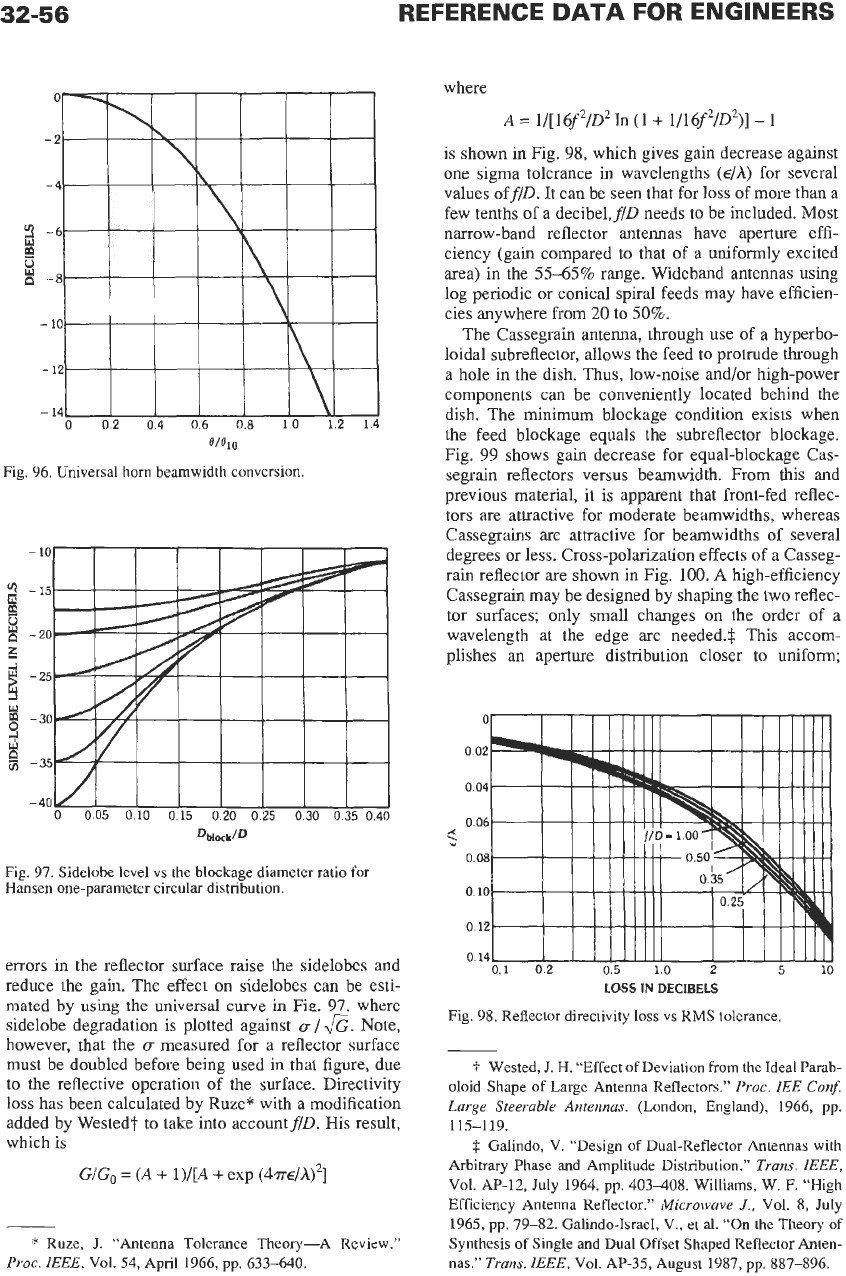
errors in the reflector surface raise the sidelobes and
reduce the gain. The effect
on
sidelobes can be esti-
mated
by
using the universal
curve
in
Fig.
97.
where
sidelobe degradation is plotted against
CT
/
&.
Note,
however, that the
CT
measured for a reflector surface
must be doubled before being used in that figure, due
to
the reflective operation
of
the surface. Directivity
loss
has been calculated by RuzeY with a modification
added by Westedt to take into account
f/D.
His result,
which is
GIG,
=
(A
+
l)/[A
+
exp
(4m/A)’]
*
Ruze,
J.
“Antenna Tolerance Theory-A Review.”
Proc.
IEEE,
Vol.
54, April 1966, pp. 633-640.
where
A
=
1/[16f2/D2 In (1
+
1/16f2/D2)]
-
1
is shown
in
Fig.
98,
which gives gain decrease against
one sigma tolerance in wavelengths
(€/A)
for several
values offlD. It can be seen that for loss
of
more than a
few tenths of a decibel,
f/D
needs to be included. Most
narrow-band reflector antennas have aperture effi-
ciency (gain compared to that of a uniformly excited
area) in the
5545%
range. Wideband antennas using
log periodic or conical spiral feeds may have efficien-
cies anywhere from
20
to
50%.
The Cassegrain antenna, through use of a hyperbo-
loidal subreflector, allows the feed to protrude through
a hole in the dish. Thus, low-noise and/or high-power
components can be conveniently located behind the
dish. The minimum blockage condition exists when
the feed blockage equals the subreflector blockage.
Fig.
99
shows gain decrease for equal-blockage Cas-
segrain reflectors versus beamwidth. From this and
previous material, it is apparent that front-fed reflec-
tors
are
attractive for moderate beamwidths, whereas
Cassegrains are attractive for beamwidths
of
several
degrees or less. Cross-polarization effects of a Casseg-
rain reflector are shown in Fig.
100.
A
high-efficiency
Cassegrain may be designed by shaping the
two
reflec-
tor surfaces; only small changes
on
the order of a
wavelength at the edge are needed.$ This accom-
plishes an aperture distribution closer to uniform;
l
I
I
I
I
IIII
I
I
Ill111~
5
10
01
02
05
10
2
LOSS
IN
DECIBELS
Fig. 98. Reflector directivity
loss
vs RMS tolerance
5.
Wested,
J.
H. “Effect of Deviation
from
the
Ideal Parab-
oloid Shape of Large Antenna Reflectors.”
Proc.
IEE
Conf.
Large Steerable Antennas.
(London, England), 1966, pp.
$
Galindo, V. “Design of Dual-Reflector Antennas with
Arbitrary Phase and Amplitude Distribution.”
Trans.
IEEE,
Vol.
Ap-12, July 1964, pp. 403408. Williams, W. F. “High
Efficiency Antenna Reflector.”
Microwave
J.,
Vol. 8, July
1965, pp. 79-82. Galindo-Israel, V., et
al.
“On the Theory
of
Synthesis
of
Single and Dual Offset Shaped Reflector Anten-
nas.”
Trans.
ZEEE,
Vol.
A€-35,
August 1987, pp. 887-896.
1
15-1 19.
ANTENNAS
32-57
overall efficiencies as high as
80%
have been reported.
However, the (corrugated) horn required
to
provide the
requisite feed pattern tends
to
provide only limited
bandwidth.
Scanning
and
Multiple-Beam
Reflectors
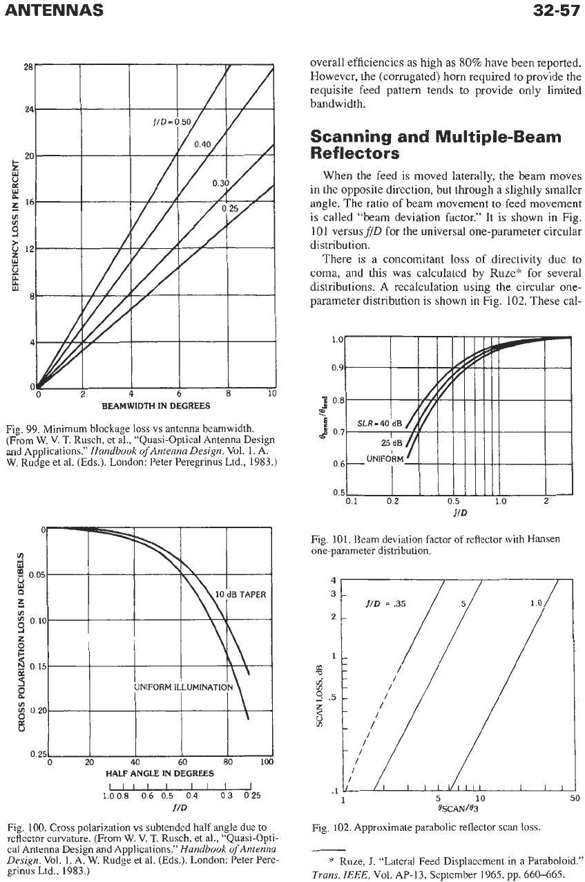
When the feed is moved laterally, the beam moves
in the opposite direction, but through a slightly smaller
angle. The ratio of beam movement to feed movement
is called “beam deviation factor.” It is shown in Fig.
101
versusflD for the universal one-parameter circular
distribution.
There is a concomitant loss of directivity due to
coma, and this was calculated by Ruze* for several
distributions.
A
recalculation using the circular one-
parameter distribution is shown in Fig.
102.
These cal-
BEAMWIDTH IN DEGREES
Fig. 99. Minimum blockage
loss
vs
antenna beamwidth.
(From
W.
V.
T.
Rusch, et
al.,
“Quasi-Optical Antenna Design
and Applications.”
Handbook
of
Antenna Design.
Vol. 1. A.
W.
Rudge et
al.
(Eds.). London: Peter Peregrinus Ltd., 1983.)
0.251
I
I I
I
I
0
20
40
60
80
100
HALF
ANGLE IN DEGREES
1111
1
11
I
I
1.00.8 0.6
0.5
0.4
0.3
0.25
f/D
Fig. 100. Cross polarization
vs
subtended half angle due to
reflector curvature. (From
W.
V.
T.
Rusch, et al., “Quasi-Opti-
cal Antenna Design and Applications.”
Handbook
of
Antenna
Design.
Vol.
1,
A.
W.
Rudge
et
al.
(Eds.). London: Peter Pere-
grinus Ltd., 1983.)
Fig. 101.
Beam
deviation factor
of
reflector with Hansen
one-parameter distribution.
BSCAN/O~
Fig. 102. Approximate parabolic reflector scan
loss.
*
Ruze,
J.
“Lateral Feed Displacement in a Paraboloid.”
Trans.
IEEE,
Vol. AP-13, September 1965, pp. 660-665.