Middleton W.M. (ed.) Reference Data for Engineers: Radio, Electronics, Computer and Communications
Подождите немного. Документ загружается.

32-28
REFERENCE
DATA
FOR ENGINEERS
TABLE
5.
PARASITIC
LENGTHS
AND
RELATIVE RESONANT FREQUENCIES
Reflector Director
Curve
Lengthlh
Resonance Lengthlh Resonance
1 0.49150
2 0.49657
3 0.50174
4 0.50702
5 0.51241
6 0.51792
0.98
0.97
0.96
0.95
0.94
0.93
0.47223
0.46764
0.46314
0.45873
0.45441
0.45016
1.02
1.03
1.04
1.05
1.06
1.07
RIM
REFLECTOR,
SUPPORT
NOT SHOWN
CROSSED
DIPOLE
Fig.
48.
Backfire antenna.
above those for conventional parabolic-reflector anten-
nas. Higher gain may be realized by feeding the
reflecting plate by a feed dipole and dipole reflector,
with a number of director dipoles between the feed
dipole and the plate.
In
this scheme, the Yagi-Uda per-
formance is combined with that of the backfire.
Frequency-Independent
Antennas
The principle of frequency-independent antennas
was established circa
1957
through
the
recognition
that conventional antenna bandwidth limitations occur
because critical dimensions change in wavelengths. An
antenna specified only in angles should then be fre-
quency independent. Of course, all antennas are of
finite size,
so
an absolute low-frequency cutoff must
exist, but within the maximum size the angular pre-
scription can be followed.*
A
commonly used fre-
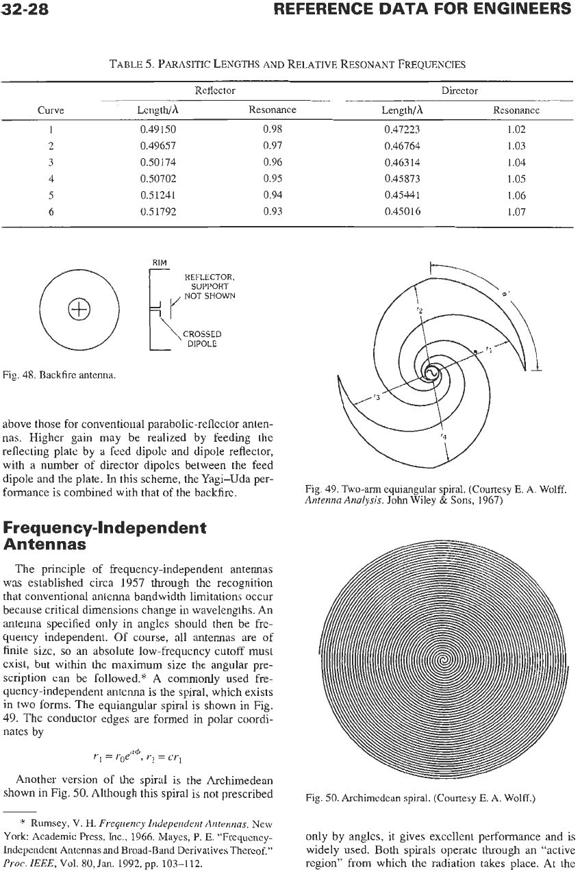
quency-independent antenna is the spiral, which exists
in two forms. The equiangular spiral is shown in Fig.
49.
The conductor edges are formed in polar coordi-
nates by
r1
=
roea4,
r2
=
crl
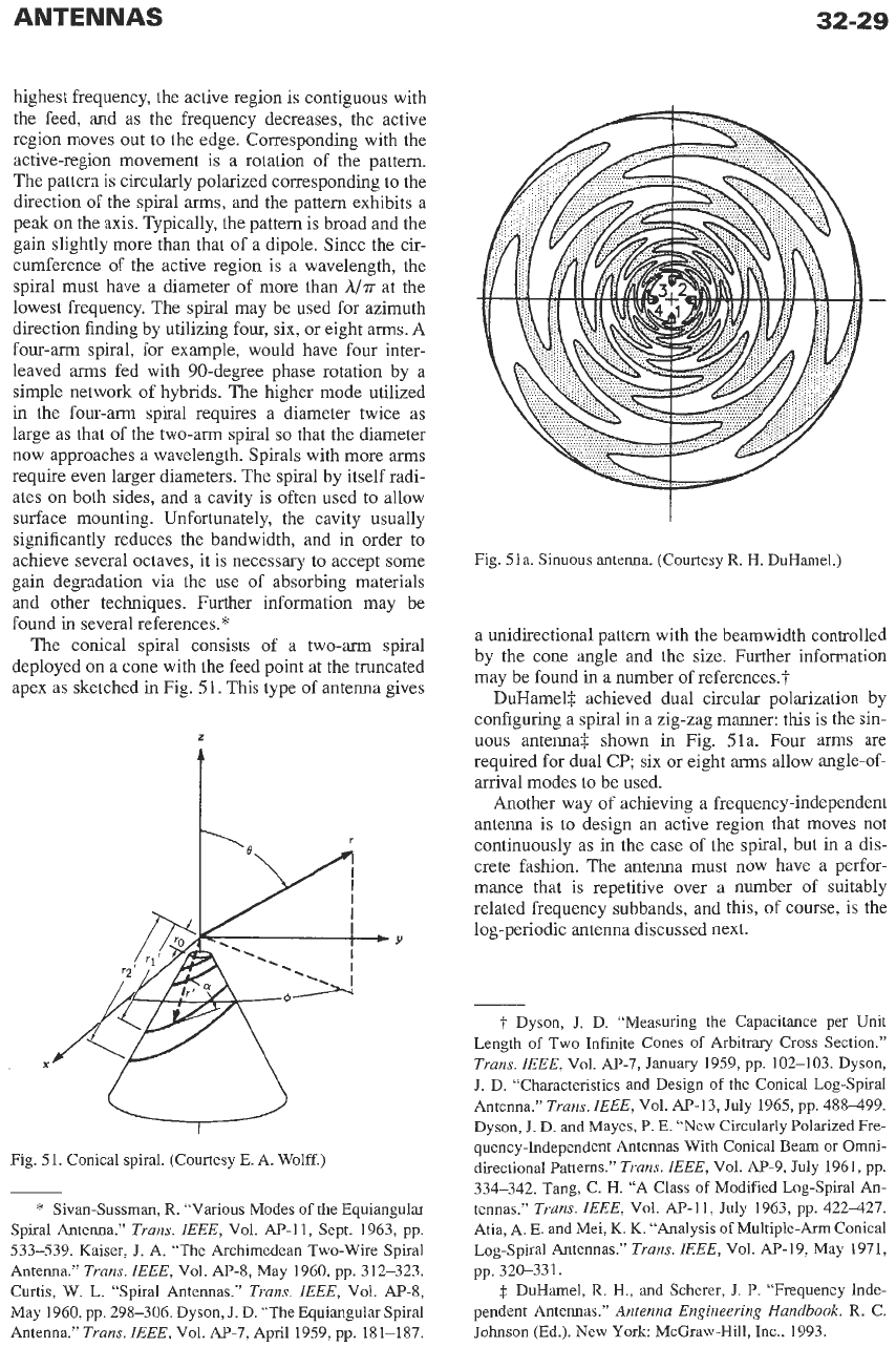
Another version of the spiral is the Archimedean
shown in Fig.
50.
Although this spiral is not prescribed
Fig.
49.
Two-arm
equiangular spiral. (Courtesy
E.
A.
Wolff.
Antenna Analysis.
John
Wiley
&
Sons,
1967)
Fig.
50.
Archimedean spiral. (Courtesy
E.
A.
Wolff.)
*
Rumsey, V.
H.
Frequency Independent Antennas.
New
York: Academic
Press,
Inc.,
1966.
Mayes,
P.
E.
“Frequency-
Independent Antennas and Broad-Band Derivatives Thereof.”
Proc.
IEEE,
Vol.
80,
Jan.
1992,
pp.
103-112.
only by angles, it gives excellent performance and is
widely used. Both spirals operate through an “active
region” from which the radiation takes place. At the
ANTENNAS
32-29
highest frequency, the active region is contiguous with
the feed, and as the frequency decreases, the active
region moves
out
to the edge. Corresponding with the
active-region movement is
a
rotation of the pattern.
The pattern is circularly polarized corresponding to the
direction of the spiral
arms,
and the pattern exhibits
a
peak on the axis. Typically, the pattern is broad and the
gain slightly more than that of
a
dipole. Since the cir-
cumference of the active region is
a
wavelength, the
spiral must have
a
diameter of more than
A/T
at the
lowest frequency. The spiral may be used for azimuth
direction finding by utilizing four, six, or eight
arms.
A
four-arm spiral, for example, would have four inter-
leaved arms fed with 90-degree phase rotation by
a
simple network of hybrids. The higher mode utilized
in the four-arm spiral requires
a
diameter twice
as
large
as
that of the two-arm spiral so that the diameter
now approaches
a
wavelength. Spirals with more arms
require even larger diameters. The spiral by itself radi-
ates on both sides, and
a
cavity is often used to allow
surface mounting. Unfortunately, the cavity usually
significantly reduces the bandwidth, and in order to
achieve several octaves, it
is
necessary to accept some
gain degradation via the use of absorbing materials
and other techniques. Further information may be
found in several references.*
The conical spiral consists of
a
two-arm spiral
deployed on
a
cone with the feed point at the truncated
apex
as
sketched in Fig.
5
1.
This type of antenna gives
z
Fig. 51. Conical spiral. (Courtesy E. A. Wolff.)
*
Sivan-Sussman,
R.
“Various Modes of the Equiangular
Spiral Antenna.”
Trans. ZEEE,
Vol. AP-11, Sept. 1963, pp.
533-539. Kaiser,
J.
A. “The Archimedean Two-Wire Spiral
Antenna.”
Trans.
IEEE,
Vol.
A€-8,
May 1960, pp. 312-323.
Curtis, W. L. “Spiral Antennas.’’
Trans. ZEEE,
Vol.
Ap-8,
May 1960, pp. 298-306. Dyson,
J.
D. “The Equiangular Spiral
Antenna.”
Trans. ZEEE,
Vol.
A€-7,
April 1959, pp. 181-187.
I
Fig. 51a. Sinuous antenna. (Courtesy
R.
H. DuHamel.)
a
unidirectional pattern with the beamwidth controlled
by the cone angle and the size. Further information
may be found in
a
number
of
references.?
DuHamelf achieved dual circular polarization by
configuring
a
spiral in
a
zig-zag manner:
this
is the sin-
uous
antenna3 shown in Fig.
51a.
Four
arms
are
required for dual
CP;
six or eight arms allow angle-of-
arrival modes
to
be used.
Another way of achieving
a
frequency-independent
antenna is to design
an
active region that moves not
continuously
as
in the case of the spiral, but in
a
dis-
crete fashion. The antenna must now have
a
perfor-
mance that is repetitive over
a
number of suitably
related frequency subbands, and this, of course, is the
log-periodic antenna discussed next.
t
Dyson,
J.
D. “Measuring
the
Capacitance per Unit
Length of Two Infinite Cones
of
Arbitrary
Cross
Section.”
Trans.
IEEE,
Vol.
AP-7,
January 1959, pp. 102-103. Dyson,
J.
D. “Characteristics and Design
of
the Conical Log-Spiral
Antenna.”
Trans.
IEEE,
Vol. AP-13, July 1965, pp. 488-499.
Dyson,
J.
D.
and
Mayes,
P.
E.
“New Circularly
Polarized
Fre-
quency-Independent Antennas With Conical
Beam
or
Omni-
directional Patterns.”
Trans.
IEEE,
Vol. A€-9, July 1961, pp.
334-342. Tang, C. H. “A Class of Modified Log-Spiral An-
tennas.”
Trans. IEEE,
Vol. AP-11, July 1963, pp. 422427.
Atia, A.
E.
and Mei, K. K. “Analysis of Multiple-Arm Conical
Log-Spiral Antennas.”
Trans.
IEEE,
Vol. AP-19, May 1971,
pp. 320-331.
$
DuHamel,
R.
H., and Scherer,
J.
P. “Frequency Inde-
pendent Antennas.”
Antenna Engineering Handbook.
R.
C.
Johnson
(Ed.).
New
York
McGraw-Hill, Inc., 1993.
32-30
REFERENCE DATA FOR ENGINEERS
Log-Periodic Antennas
Although the term “log-periodic” can be applied to
any antenna designed with a structure that is periodic
in
the logarithm of some normalized dimensions,
almost all log-periodic antennas
in
use
are
of the
dipole-array type or of the trapezoidal-tooth type.
Common usage now calls these simply “log-periodic
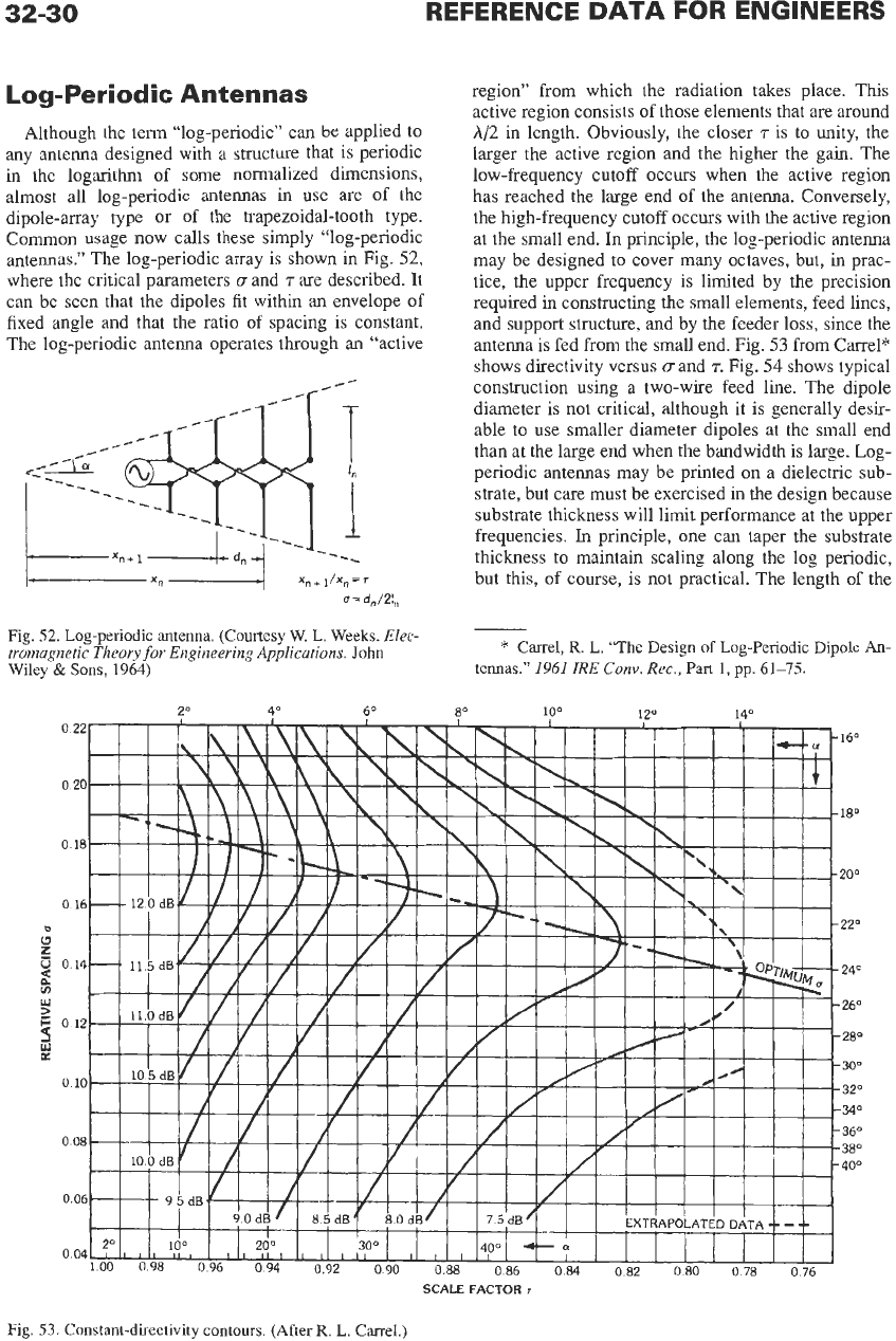
antennas.” The log-periodic array is shown in Fig.
52,
where the critical parameters
(T
and
r
are described. It
can be seen that the dipoles fit within an envelope of
fixed angle and that the ratio of spacing is constant.
The log-periodic antenna operates through an “active
region” from which the radiation takes place.
This
active region consists of those elements that are around
A/2
in length. Obviously, the closer
T
is to unity, the
larger the active region and
the
higher the gain. The
low-frequency cutoff occurs when the active region
has reached the large end of the antenna. Conversely,
the high-frequency cutoff occurs with the active region
at the small end. In principle, the log-periodic antenna
may be designed to cover many octaves, but, in prac-
tice, the upper frequency is limited by the precision
required in constructing
the
small elements, feed lines,
and support structure, and by
the
feeder loss, since the
antenna is fed
from
the small end. Fig.
53
from Carrel”
shows directivity versus
u
and
r.
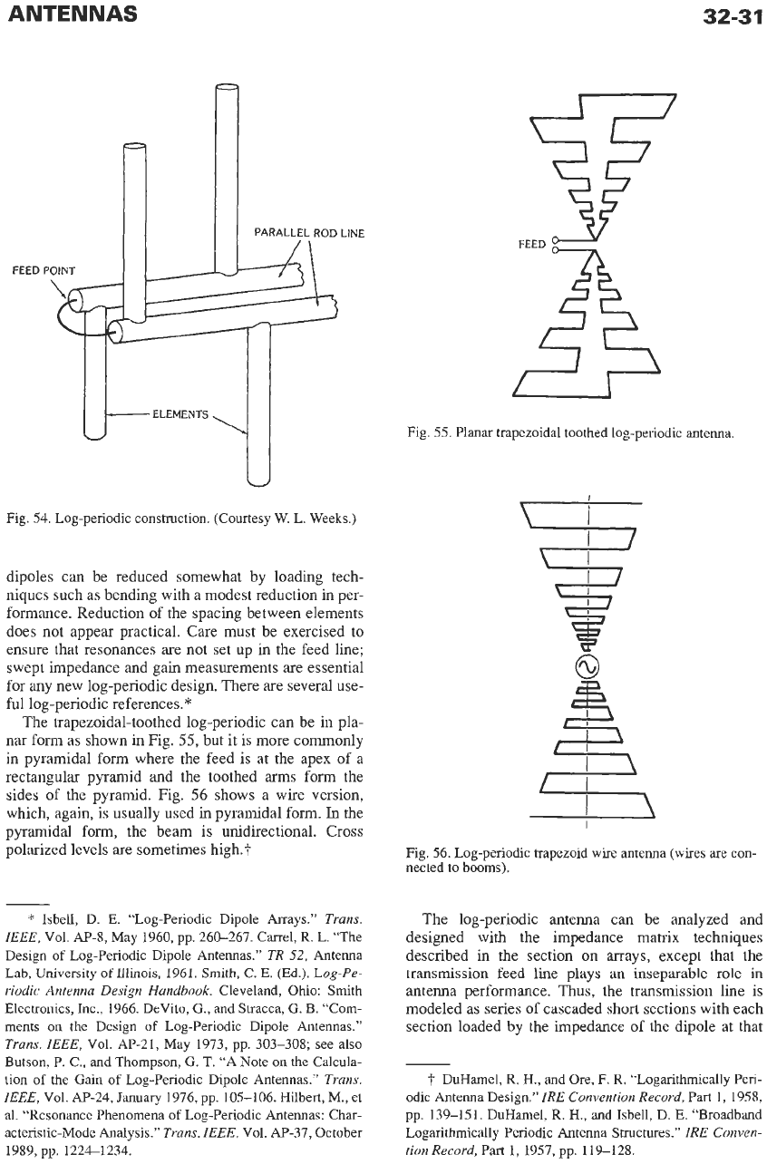
Fig.
54
shows typical
construction using a two-wire feed line. The dipole
diameter is
not
critical, although it
is
generally desir-
able to use smaller diameter dipoles at the small end
than at the large end when the bandwidth is large. Log-
periodic antennas may be printed
on
a dielectric sub-
strate, but care must be exercised in the design because
substrate thickness will limit performance at the upper
frequencies.
In
principle, one can taper the substrate
thickness to maintain scaling along the log periodic,
but this, of course, is not practical. The length of the
Fig.
52.
Log-periodic antenna. (Courtesy W.
L.
Weeks.
Elec-
tromagnetic Theory
for
Engineering Applications.
John
Wiley
&
Sons,
1964)
*
Carrel,
R.
L.
“The
Design
of
Log-Periodic Dipole
AI-
tennas.”
1961
IRE
Conv. Rec.,
Part
1,
pp.
61-15.
0
22
0
20
0
18
0 16
m
0
z
3
014
8
3
F
012
0
10
0
08
0
06
0 04
SCALE
FACTOR
r
Fig.
53.
Constant-directivity contours. (After
R.
L. Carrel.)
ANTENNAS
32-31
FEED
POINT
JL-4
‘A
PARALLEL
ROD
LINE
-4
-ELEMENTS
U
3
Fig. 54. Log-periodic construction. (Courtesy
W.
L.
Weeks.)
dipoles can be reduced somewhat by loading tech-
niques such as bending with a modest reduction in per-
formance. Reduction
of
the spacing between elements
does not appear practical. Care must be exercised
to
ensure that resonances are not set
up
in the feed line;
swept impedance and gain measurements are essential
for any new log-periodic design. There are several use-
ful log-periodic references.”
The trapezoidal-toothed log-periodic can be in pla-
nar form as shown in Fig.
55,
but it is more commonly
in pyramidal form where the feed is at the apex
of
a
rectangular pyramid and the toothed
arms
form the
sides
of
the pyramid. Fig.
56
shows a wire version,
which, again, is usually used
in
pyramidal form.
In
the
pyramidal form, the beam is unidirectional. Cross
polarized levels are sometimes high.?
*
Isbell,
D.
E.
“Log-Periodic Dipole Arrays.”
Trans.
IEEE,
Vol. Ap-8, May 1960, pp. 260-267. Carrel, R.
L.
“The
Design
of
Log-Periodic Dipole Antennas.”
TR
52,
Antenna
Lab, University
of
Illinois,
1961. Smith,
C.
E.
(Ed.). Log-Pe-
riodic Antenna Design Handbook.
Cleveland, Ohio: Smith
Electronics, Inc., 1966. DeVito,
G.,
and Stracca,
G.
B.
“Com-
ments
on
the
Design
of
Log-Periodic Dipole Antennas.”
Trans.
IEEE,
Vol. AP-21, May 1973, pp. 303-308;
see
also
Butson, P.
C.,
and Thompson,
G.
T.
“A Note
on
the
Calcula-
tion of the Gain of Log-Periodic Dipole Antennas.”
Trans.
IEEE,
Vol. AP-24,
January
1976, pp. 105-106. Hilbert, M., et
al.
“Resonance Phenomena
of
Log-Periodic Antennas: Char-
acteristic-Mode Analysis.”
Trans.
IEEE,
Vol. AP-37, October
1989, pp. 1224-1234.
37
25
Fig. 55. Planar trapezoidal toothed log-penodic antenna.
I
r
\
I
Fig. 56. Log-periodic trapezoid
wire
antenna
(wires
are con-
nected to booms).
The log-periodic antenna can be analyzed and
designed with the impedance matrix techniques
described in the section
on
arrays, except that the
transmission
feed line plays
an
inseparable role
in
antenna performance.
Thus,
the transmission line is
modeled as series of cascaded short sections with each
section loaded by the impedance of the dipole at that
7
DuHamel,
R.
H.,
and Ore,
F.
R. “Logarithmically Pen-
odic Antenna Design.”
IRE Convention Record,
Part
1,
1958,
pp. 139-151.
DuHamel,
R.
H.,
and Isbell, D.
E.
“Broadband
Logarithmically Periodic Antenna Structures.”
IRE Conven-
tion Record,
Part
1,
1957, pp. 119-128.
32-32
point
on
the feeder. Of course, the dipole impedance
includes all mutual impedances. This results in a trans-
mission-line transformation matrix that is solved in
conjunction with the dipole-array impedance matrix. It
has been found that although the current distribution
on
the active-region elements is nearly sinusoidal, ele-
ments on either side may have significantly different
current distributions. Thus, for accurate results, it is
necessary to use either moment method segmentation
on the dipoles or to use the three-term current theory
of Chang.*
The
latter is simpler and gives quite satis-
factory results.
Fractal Antennas
Fractal theory has been applied to antennas but the
results have not been promising. Many parts of nature
are well modeled by fractals, e.g. certain ferns; unf‘or-
tunately Maxwell’s equations are not fractal. To see
this, consider frequency independent antennas such as
the planar spiral and the log-periodic dipole array.
High frequency active regions are small and located at
(near) the feed; low frequency active regions are large
and are located farthest from the feed. Thus, feed cur-
rents can activate large active regions with only minor
effects in passing through the intervening smaller
regions.
In
contrast, the classic Mandelbrot fractal dia-
gram? has one (largest) blob where the feed would be,
with more smaller blobs on the large blob periphery;
each smaller blob has its own cluster of still smaller
blobs, etc. This topology is just the inverse of the fre-
quency independent antenna topology. Generally, a
conventional antenna in the same area (volume) per-
forms better.
ARRAYS
General Characteristics
Arrays of antenna elements are almost always regu-
larly spaced on a rectangular or triangular lattice for
planar arrays, equally spaced for linear arrays. Non-
uniformly spaced (thinned) arrays will be discussed
later. Since fields add, the pattern of an array is the
product of the element pattern and the array factor, the
latter being that of an array of isotropic elements.
Thus,
the element and array behavior can be separated
for pattern purposes. The array factor for N elements
can be written:
ll=l
*
Chang, D. C.,
Lee,
S.
W., and Rispin,
L.
“Simple For-
mula for Current on a Cylindrical Receiving Antenna.”
Trans.
ZEEE,
Vol.
AP-26,
September 1978, pp. 683690.
t
Pentgen,
H. O.,
and Saupe,
D.
The Science
of
Fractals.
New York: John Wiley
&
Sons, 1997.
where
u
=
rr(d/h)
sin
8
cos
4
uo
=
rr(d/h)
sin
8,
cos
4o
The interelement phase shift,
u,,,
positions the beam
at
eo,
&.
Element spacing is
d,
and the excitation coef-
ficients
are
A,.
Symmetric arrays can be written as a
real series with terms
A,,
cos
n(u
-
uo).
Factoring
the
array expression displays the zeros in
u;
these
are
of
critical importance
in
controlling array-factor behav-
ior. Uniform excitation gives a sin
mlm
or sinc
rn~
pattern, and this is both a constituent of a shaped beam
pattern (using Woodward-Lawson synthesis$) and a
prototype for low-sidelobe designs. Zeros of sinc
m
occur at
u
=
+n;
shifting these zeros controls the side-
lobe envelope. Although in the early years of antennas,
array and aperture excitation functions were chosen
for simplicity and integrability, they are now designed
through zero placement to yield optimum performance
given the requirements. Computer codes are then
employed to furnish needed details. Large arrays,
roughly N of
20
or more,
are
usually designed by sam-
pling a continuous distribution. See the section
on
aperture distributions. For small arrays, the zeros of a
polynomial, such as the Chebyshev, are adjusted; the
order of the polynomial matches the number of ele-
ments in the array.§ For all types of arrays, design
using physical principles of zero placement should be
used to obtain optimum performance.” This also obvi-
ates comparing various well established but meretri-
cious arraylaperture distributions.
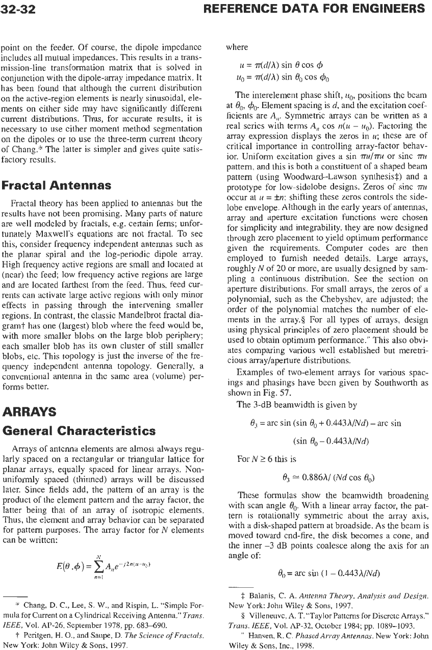
Examples of two-element arrays for various spac-
ings and phasings have been given by Southworth as
shown in Fig.
57.
The 3-dB beamwidth is given by
8,
=
arc sin (sin
0,
+
0.443hINd)
-
arc
sin
(sin
0,
-
0.443hINd)
For N
2
6
this is
0,
=
0.886hI
(Nd
cos
8,)
These formulas show the beamwidth broadening
with scan angle
8,.
With a linear array factor, the pat-
tern
is
rotationally symmetric about the array
axis,
with a disk-shaped pattern at broadside. As the beam is
moved toward end-fire, the disk becomes a cone, and
the inner
-3
dB points coalesce along the axis for an
angle
of
8,
=
arc
sin
(1
-
0.443hINd)
$
Balanis, C.
A. Antenna Theory, Analysis and Design.
5
Villeneuve,
A.
T.
“Taylor Patterns for Discrete Arrays.”
’’
Hansen,
R.
C.
PhasedArruy Antennas.
New York
John
New York:
John
Wiley
&
Sons,
1997.
Trans.
ZEEE,
Val.
A€-32,
October 1984; pp. 1089-1093.
Wiley
&
Sons, Inc., 1998.
ANTENNAS
32-33
SEPARATION
n
x/4
x/2
3x/4
x
Fig.
57.
Patterns of two-element arrays. (From Southworth,
G.
C.
“Certain
Factors
Affecting
the
Gain
of
Directive Antenna
Arrays.”
Proc.
IRE,
Vol.
18,
Sept.
1930,
pp.
1502-1536.)
For beam angles beyond this angle, a single end-fire
beam exists. At end-fire, the beamwidth is larger than
broadside beamwidth by the factor:
endfire
1
broadside
zrO886hlo
When analog phasers are used to produce the inter-
element phase shift,
uo,
required to scan the beam, any
beam position may be reached if the phasers can be set
precisely. Digital phasers, however, have
a
least count
of phase shift, and the array positioning will similarly
have a least position change.
An m-bit phaser has
a
least count phase shift of
4c
=
2n-12”
and this produces
a
least beam shift
of
kd
sine,,,
k
=
2.rr/h.
These are related by
kd
sin
e,,
=
~/2”-‘
For the common A12-spaced array, the relationship
is sin
e,,
=
2”*-’.
Table
6
shows the fineness
of
beam
steering available versus the number
of
bits per phaser.
Pseudo-randomization can reduce the pointing error.*
*
Smith,
M.
S., and
Guo,
Y.
C. “A Comparison
of
Meth-
ods for Randomizing Phase Quantization Errors in Phased
Ar-
rays.”
Trans.
IEEE,
Vol.
AI-31,
November
1983,
pp.
821-
827.
TABLE
6.
FINENESS
OF
BEAM STEERING
m
e,,
(degrees)
30
14.48
7.18
3.58
1.79
Positioning the beam
of
an array at one frequency
requires only a phaser per element. Positioning the
beam over a large bandwidth requires the proper time
delay, i.e., line length, at each element. The bandwidth
allowed with the use
of
phasers depends on array size;
bandwidth is taken
as
beam movement to the -3-dB
point:
=
(sin 0,
-
sin 8Jsin
8,
=
Al2L
sin
0’
Assumed here is a not small array length. For a
beam angle of 30 degrees, for example, the fractional
bandwidth is
BW
=
AIL
Thus, long arrays have less bandwidth in terms
of
beam shift at the band edges.
32-34
REFERENCE
DATA
FOR ENGINEERS
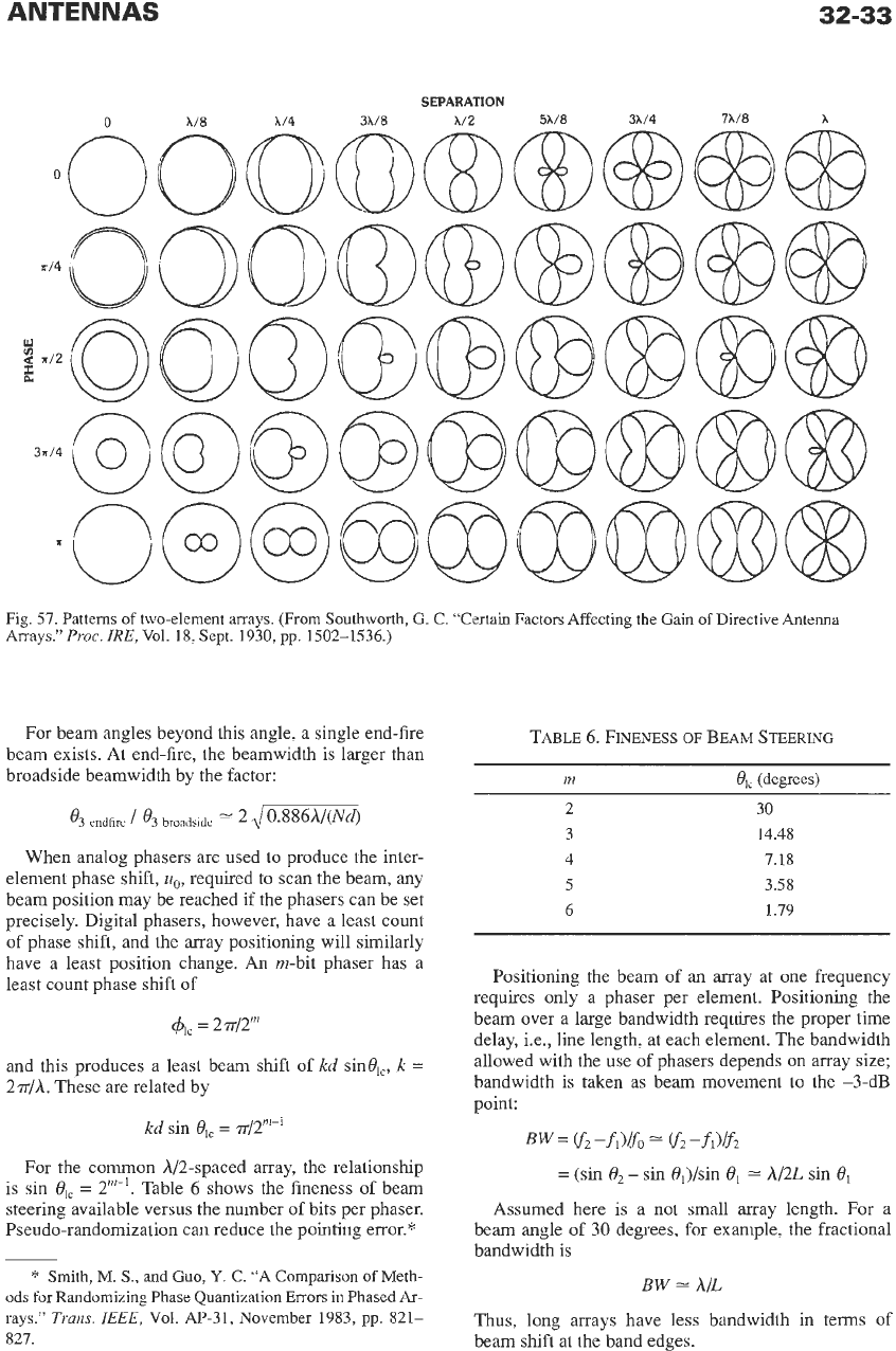
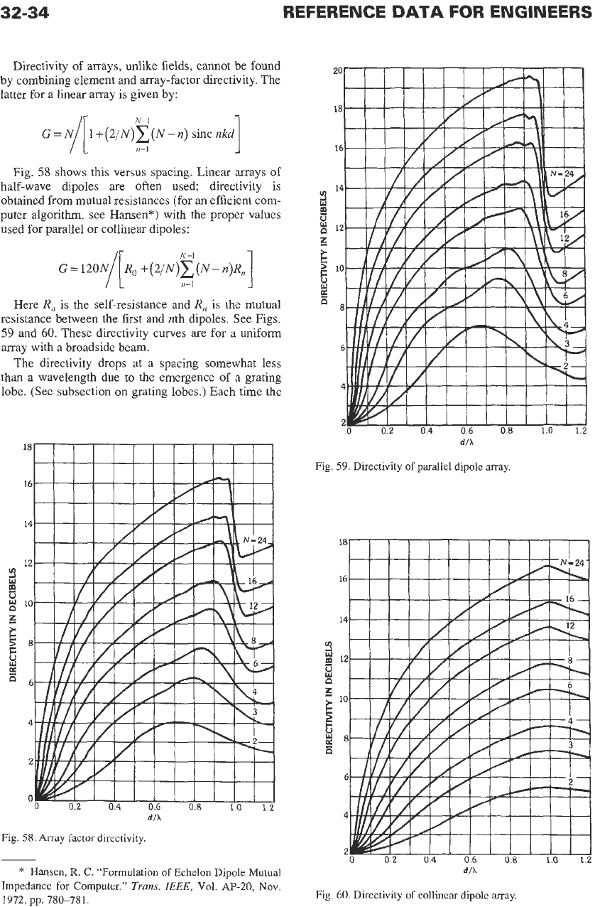
Directivity of arrays, unlike fields, cannot be found
by combining element and array-factor directivity. The
latter for a linear array is given by:
1
Fig.
58
shows this versus spacing. Linear arrays of
half-wave dipoles are often used; directivity is
obtained from mutual resistances (for an efficient com-
puter algorithm, see Hansen”) with the proper values
used for parallel or collinear dipoles:
1
Here
R,
is the self-resistance and
R,
is the mutual
resistance between the first and nth dipoles. See Figs.
59
and
60.
These directivity curves are for a uniform
array with a broadside beam.
The directivity drops at
a
spacing somewhat less
than a wavelength due to the emergence of a grating
lobe. (See subsection on grating lobes.) Each time the
0
0.2
0.4
0.6
0.8
1.0
1.2
d/X
Fig.
58.
Array factor directivity.
*
Hansen,
R.
C.
“Formulation of Echelon Dipole Mutual
Impedance for Computer.”
Trans.
IEEE,
Vol.
AP-20,
Nov.
1972,
pp.
780-781.
dIX
Fig.
59.
Directivity of parallel dipole array.
0
0.2
04
06 08
1.0
1.2
dlh
60.
Directivity of collinear dipole array.
ANTENNAS
32-35
spacing is increased enough to admit another grating
lobe, the gain drops proportionately. Directivity of pla-
nar arrays can be approximated in lieu of exact calcu-
lations, by computing the gain of constituent
x-
and
y-
direction linear arrays of the exact elements, multiply-
ing these directivities together, and then adding a cor-
rection factor.* Since dipole directivity of
1.604
is
included twice. it must be divided out.
Grating and Quantization
Lobes
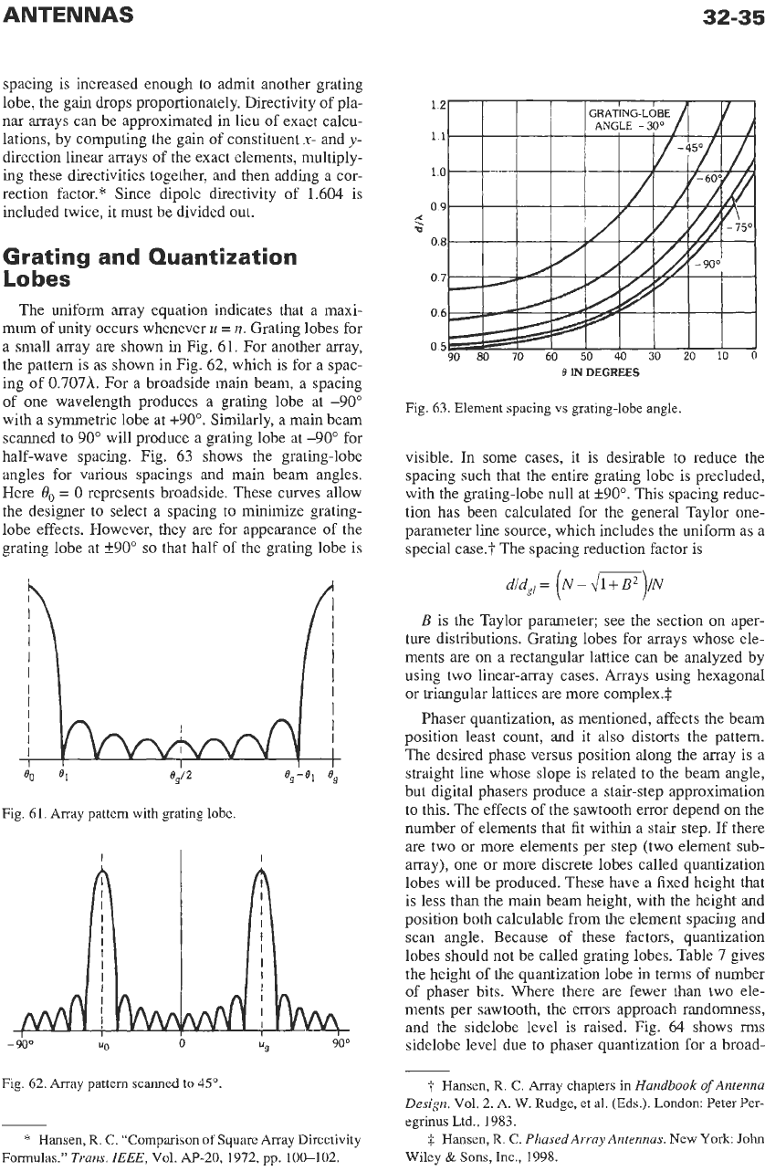
The uniform array equation indicates that a maxi-
mum of unity occurs whenever
u
=
n.
Grating lobes for
a small array are shown in Fig.
61.
For another array,
the pattern is as shown in Fig.
62,
which is for a spac-
ing of
0.707h.
For a broadside main beam, a spacing
of one wavelength produces a grating lobe at
-90"
with a symmetric lobe at
+90".
Similarly, a main beam
scanned to
90"
will produce a grating lobe at
-90"
for
half-wave spacing. Fig.
63
shows the grating-lobe
angles for various spacings and main beam angles.
Here
19,
=
0
represents broadside. These curves allow
the designer to select a spacing to minimize grating-
lobe effects. However, they are for appearance of the
grating lobe at
+90° so
that half of the grating lobe is
n
Ii
Fig. 61. Array pattern with grating
lobe.
i
I
I
-
900
"0
b
"Ll
90D
Fig. 62. Array pattern scanned
to
45".
*
Hansen,
R.
C. "Comparison
of
Square Array Directivity
Formulas."
Trans.
IEEE,
Vol. AP-20, 1972, pp. 100-102.
0
IN
DEGREES
Fig. 63. Element spacing vs grating-lobe angle.
visible.
In
some cases, it is desirable to reduce the
spacing such that the entire grating lobe is precluded,
with the grating-lobe null at
k90".
This spacing reduc-
tion has been calculated for the general Taylor one-
parameter line source, which includes the uniform as a
special case.? The spacing reduction factor is
dld,,
=
(N
-
m)/N
B
is the Taylor parameter; see the section on aper-
ture distributions. Grating lobes for arrays whose ele-
ments
are
on a rectangular lattice can be analyzed by
using two linear-array cases. Arrays using hexagonal
or triangular lattices are more complex.$
Phaser quantization, as mentioned, affects the beam
position least count, and it also distorts the pattern.
The desired phase versus position along the array is a
straight line whose slope is related to the beam angle,
but digital phasers produce a stair-step approximation
to this. The effects of the sawtooth error depend
on
the
number of elements that fit within a stair step. If there
are
two or more elements per step (two element sub-
array), one or more discrete lobes called quantization
lobes will be produced. These have a fixed height that
is less than the main beam height, with the height and
position both calculable from the element spacing and
scan angle. Because of these factors, quantization
lobes should not be called grating lobes. Table
7
gives
the height of the quantization lobe in terms of number
of
phaser bits. Where there are fewer than two ele-
ments per sawtooth, the errors approach randomness,
and the sidelobe level is raised. Fig.
64
shows rms
sidelobe level due to phaser quantization for a broad-
7
Hansen,
R. C.
Array chapters in
Handbook
of
Antenna
Design.
Vol.
2.
A.
W. Rudge, et al. (Eds.). London: Peter Per-
egrinus Ltd., 1983.
i.
Hansen,
R.
C.
PhasedArray Antennas.
New York:
John
Wiley
&
Sons, Inc., 1998.
32-36
REFERENCE
DATA
FOR ENGINEERS
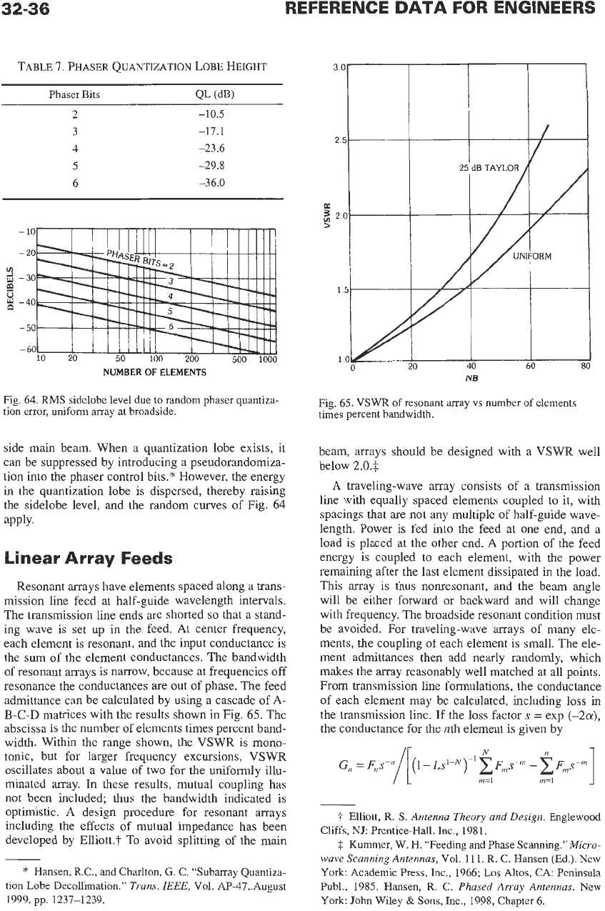
TABLE
7.
PHASER
QUANTIZATION
LOBE HEIGHT
2 -10.5
3 -17.1
4 -23.6
5 -29.8
6 -36.0
-
10
-
20
"
-30
I?
8
g
-40
-
50
-
60
NUMBER
OF
ELEMENTS
Fig. 64. RMS sidelobe level due to random phaser quantiza-
tion error, uniform array at broadside.
side main beam. When a quantization lobe exists, it
can be suppressed by introducing a pseudorandomiza-
tion into
the
phaser control bits.* However, the energy
in
the quantization lobe is dispersed, thereby raising
the sidelobe level, and the random curves of Fig.
64
apply.
Linear Array Feeds
Resonant arrays have elements spaced along a
trans-
mission line feed at half-guide wavelength intervals.
The transmission line ends are shorted
so
that a stand-
ing wave is set up
in
the feed. At center frequency,
each element is resonant, and the input conductance is
the sum of the element conductances. The bandwidth
of resonant arrays is narrow, because at frequencies
off
resonance the conductances are out
of
phase. The feed
admittance can be calculated by using a cascade of A-
B-C-D
matrices with the results shown in Fig.
65.
The
abscissa is the number of elements times percent band-
width. Within the range shown, the
VSWR
is mono-
tonic, but for larger frequency excursions,
VSWR
oscillates about a value of two for
the
uniformly illu-
minated array. In these results, mutual coupling has
not been included; thus the bandwidth indicated is
optimistic.
A
design procedure for resonant arrays
including the effects of mutual impedance has been
developed by Elliott.? To avoid splitting of the main
*
Hansen, R.C., and Charlton,
G.
C. "Subarray Quantiza-
tion Lobe Decollimation."
Trans.
ZEEE,
Vol. A€-47,.August
1999, pp. 1237-1239.
0
20
40
60
80
NB
Fig. 65.
VSWR
of
resonant array vs number of elements
times percent bandwidth.
beam, arrays should be designed with a
VSWR
well
below
2.04
A traveling-wave array consists
of
a transmission
line with equally spaced elements coupled to it, with
spacings that
are
not any multiple of half-guide wave-
length. Power is fed into the feed at one end, and a
load is placed at the other end. A portion of the feed
energy is coupled to each element, with the power
remaining after the last element dissipated
in
the load.
This array is thus nonresonant, and the beam angle
will be either forward or backward and will change
with frequency. The broadside resonant condition must
be avoided. For traveling-wave arrays of many ele-
ments, the coupling of each element is small. The ele-
ment admittances then add nearly randomly, which
makes the array reasonably well matched at all points.
From transmission line formulations, the conductance
of each element may be calculated, including
loss
in
the transmission line.
If
the loss factors
=
exp
(-2cr),
the conductance for the nth element is given by
t
Elliott,
R.
S.
Antenna Theory and Design.
Englewood
Cliffs,
NJ:
Prentice-Hall, Inc., 1981.
i.
Kummer, W. H. "Feeding and Phase Scanning."
Micro-
wave Scanning Antennas,
Vol. 11
1.
R.
C. Hansen (Ed.). New
York: Academic Press, Inc., 1966;
Los
Altos,
CA: Peninsula
Publ., 1985. Hansen,
R.
C.
Phased Array Antennas.
New
York John Wiley
&
Sons,
Inc., 1998, Chapter 6.
ANTENNAS
32-37
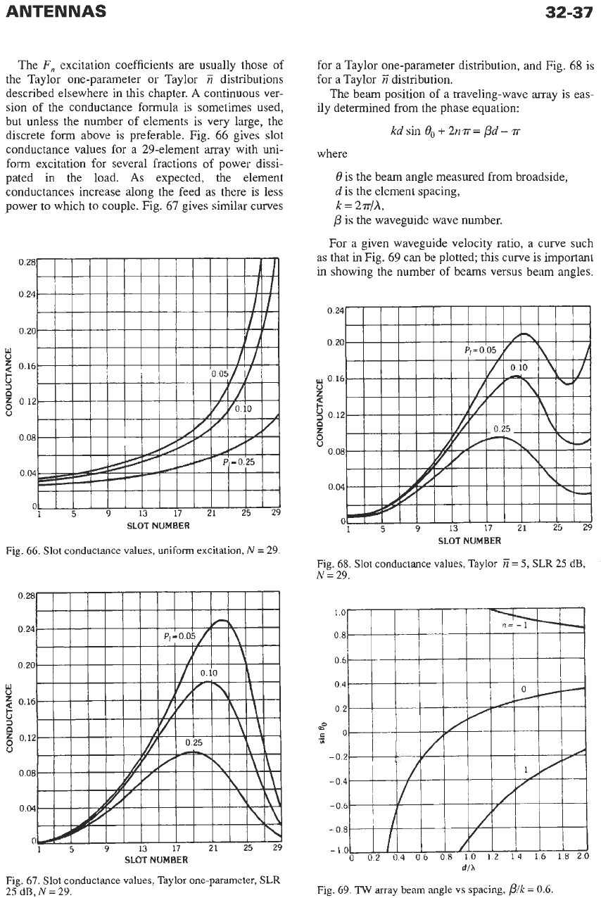
The
F,
excitation coefficients are usually those of
the Taylor one-parameter or Taylor
E
distributions
described elsewhere in this chapter.
A
continuous ver-
sion
of
the conductance formula is sometimes used,
but unless the number of elements is very large, the
discrete form above is preferable. Fig. 66 gives slot
conductance values for a 29-element array with uni-
form excitation for several fractions of power dissi-
pated
in
the load.
As
expected, the element
conductances increase along the feed as there is less
power to which to couple. Fig. 67 gives similar curves
0 28
0
24
0 20
w
016
0
z
012
8
0
08
0
04
0
SLOT
NUMBER
Fig.
66.
Slot conductance values, uniform excitation,
N
=
29.
SLOT
NUMBER
Fig.
67.
Slot conductance values, Taylor one-parameter,
SLR
25 dB,
N
=
29.
for a Taylor one-parameter distribution, and Fig. 68 is
for a Taylor
E
distribution.
The beam position of
a
traveling-wave array is eas-
ily determined from the phase equation:
kd
sin
0,
+
2n~=
pd-
T
where
0
is the beam angle measured from broadside,
d
is the element spacing,
k
=
2?r/A,
p
is the waveguide wave number.
For a given waveguide velocity ratio, a curve such
as that
in
Fig. 69 can be plotted; this curve is important
in
showing the number of beams versus beam angles.
SLOT
NUMBER
Fig.
68.
Slot
conductance values, Taylor
E=
5,
SLR
25 dB,
N
=
29.
dlh
Fig. 69. TW array beam angle vs spacing,
plk
=
0.6.