Muga G. Time in Quantum Mechanics - Vol. 2
Подождите немного. Документ загружается.

6 The Quantum Jump Approach and Some of Its Applications 153
occurred until time t. The normalization is chosen in such a way that the trace gives
the relative size of the subensemble. To begin with, in the time interval [t
0
, t
0
+Δ],
a photon will have been detected for some of the atoms, i.e., there will have been a
jump on some trajectories, and this subensemble is described by Rρ(t
0
)Δt, includ-
ing its relative size. The complementary subensemble is described by the difference
of the original ρ(t
0
+Δt) and Rρ(t
0
)Δt, so that
ρ
0
(t
0
+Δt) = ρ(t
0
+Δt) − Rρ(t
0
)Δt . (6.108)
This subensemble as a total would evolve until t
0
+ 2Δt with the Bloch equations,
i.e., as T
B
(t
0
+ 2Δt, t
0
+ Δt) ρ
0
(t + Δt), and the sub-subensemble with no photon
detected at time t +2Δt is again a difference,
ρ
0
(t
0
+2Δt) = T
B
(t
0
+2Δt, t
0
+Δt)ρ
0
(t
0
+Δt) −Rρ
0
(t
0
+Δt)Δt . (6.109)
In the same vain one obtains for general t
ρ
0
(t +Δt) = T
B
(t +Δt, t) ρ
0
(t) −Rρ
0
(t) Δt . (6.110)
If L
B
denotes the superoperator which generates the time development of the Bloch
equations, then T
B
(t +Δt, t) = e
L
B
Δt
and (6.110) can be written as
ρ
0
(t +Δt) = (1 +L
B
Δt) ρ
0
(t) −Rρ
0
(t) Δt . (6.111)
This finally yields for the subensemble with no jump (photon detection) until time t
the equation
˙ρ
0
(t) =
L
B
−R
ρ
0
(t) . (6.112)
The difference in the brackets is just the time development given by the conditional
Hamiltonian, as seen from (6.94).
It may seem from this derivation that one might be able to take the limit Δt → 0
without running into the quantum Zeno effect. However, it is well known that the
optical Bloch equations are not valid for arbitrarily small times because also in their
derivation the Markov property is used, and this requires Δt to be larger than the
correlation time. Hence for Δt → 0 one would have difficulties with (6.111).
6.5.3 Connection with Continuous Measurements
In order to describe continuous measurements, Davies and Srinivas [47, 48] have
extended the axiomatics of quantum mechanics by postulates for “homogeneous
quantum counting processes.” In particular, their postulates imply the existence
of two superoperators, J and S
t
, which map trace class operators to trace class
154 G.C. Hegerfeldt
operators and satisfy certain properties. For an individual system of an ensem-
ble described by a density matrix ρ their meaning is as follows. tr(S
t
ρ)isthe
probability of finding no counting event in [0, t], and the probability density,
w
DS
(t
1
,...,t
n
;[0, t]), for finding a counting event exactly at the times t
1
,...,t
n
in [0, t] is given by
w
DS
(t
1
,...,t
n
;[0, t]) = tr
S
t−t
n
JS
t
n
−t
n−1
J ··· JS
t
2
−t
1
JS
t
1
ρ
. (6.113)
For a particular system J and S
t
have to be determined phenomenologically or by
intuition.
A comparison with (6.98) shows that this has the same structure as that obtained
by the QJA and that the unknown superoperators J and S
t
have to coincide with
the R and T
cond
constructed above. In contrast to the axiomatic theory of Davies
and Srinivas, however, the superoperators are explicitly known in the QJA. In
this way one has arrived, without the need of new axioms, at the results of the
continuous measurement theory of [47, 48] for the general N-level atom within
the usual framework of quantum mechanics and with the reduction rule of von
Neumann and L
¨
uders for demolition measurements, except that a temporal coarse
graining has been used. Counting processes analogous to (6.99) have also been
derived in [44].
6.6 How to Replace Density Matrices by Pure States
in Simulations
In many cases the reset state is not a pure state even if one starts in a pure state.
Moreover, the particular reset state in a quantum trajectory may depend on the
conditional state preceding it and thus on the whole history before the resetting.
If in a simulation one would work with density matrices instead of pure states,
one would enormously complicate the numerics for large dimension N of the level
space since density matrices lead to N
2
instead of N , as pointed out in Sect. 6.4.3.
It will be shown elsewhere [26] that for simulations one can always go over to
quantum trajectories with pure states which yield both the same jump statistics and
the Bloch equations as the original trajectories. In simple situations this procedure
has been used before [4]. For simulations this is of great numerical advantage if N is
large. The general proof of this statement is somewhat involved and it may be more
instructive to see how this works in a specific example which is simple enough but
still exhibits all salient features.
To this end we consider a simple three-level cascade system as in Fig. 6.7, where
level 2 may decay to level 1 and level 3 to level 2. Only the 1–3 transition is driven
by a laser. To keep things simple we assume the laser to be on resonance, i.e., ω
L
=
ω
3
−ω
1
. In the Schr
¨
odinger picture the conditional Hamiltonian is then of the form

6 The Quantum Jump Approach and Some of Its Applications 155
H
cond
=
3
1
ω
i
|ii|+
Ω
2
|13|e
iω
L
t
+|31|e
−iω
L
t
−
iA
2
2
|22|−
iA
2
|33| ,
(6.114)
where A
2
and A are the Einstein coefficients of level 2 and 3, respectively. By going
over to the interaction picture we get rid of the time dependence and obtain
H
I
cond
=
Ω
2
|13|+|31|
−
iA
2
2
|22|−
iA
2
|33| .
(6.115)
The reset operation for this system is given in (6.89), and here we write it in the
form
Rρ = A
2
ρ
22
|11|+Γρ
23
|12|
+Γ
∗
ρ
32
|21|+Aρ
33
|22| ,
(6.116)
where we use the abbreviation Γ ≡ Γ
1332
+ Γ
3213
. Note that |Γ |
2
≤ A
2
A so that
Rρ is a positive operator.
The operator H
I
cond
consists of the part −i(A
2
/2)|22|, responsible for the
decay of level 2, and a remainder operating in the 2D subspace spanned by |1
and |3.Ifλ
±
denote the eigenvalues of the 2D part, i.e.,
λ
±
=−
iA
4
±
1
4
/
4Ω
2
− A
2
,
(6.117)
then the conditional time development in the interaction picture is easily determined
as in (6.40) to be given by
exp{−iH
I
cond
t/}=e
−A
2
t/2
|22|
+
2
√
4Ω
2
− A
2
e
−iλ
+
t
Ω
2
|13|+|31|
!
−λ
−
|11|−
λ
−
+
iA
2
!
|33|
−e
−iλ
−
t
Ω
2
|13|+|31|
!
−λ
+
|11|−
λ
+
+
iA
2
!
|33|
.
(6.118)
In particular, one finds
exp{−iH
I
cond
t/}|1=
2
√
4Ω
2
− A
2
e
−iλ
+
t
−λ
−
|1+
Ω
2
|3
−e
−iλ
−
t
−λ
+
|1+
Ω
2
|3
,
exp{−iH
I
cond
t/}|2=e
−A
2
t/2
|2 .
(6.119)
156 G.C. Hegerfeldt
For an initial state |α the probability density, denoted by w
1
(t, t
0
= 0; |α), for the
first photon is, by (6.38),
w
1
(t, t
0
= 0; |α) =
i
α|exp{iH
†
cond
t/}
H
cond
− H
†
cond
exp{−iH
cond
t/}|α .
(6.120)
For a superposition of |1 and |2,
|α=α
1
|1+α
2
|2 , (6.121)
one then obtains
w
1
(t, t
0
=0; |α)=|α
2
|
2
A
2
e
−A
2
t
+|α
1
|
2
4AΩ
2
4Ω
2
− A
2
e
−At/2
sin
1
4
/
4Ω
2
− A
2
t
2
.
(6.122)
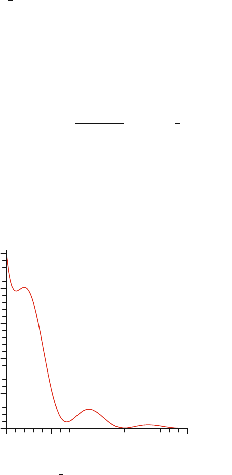
Figure 6.8 shows the behavior of w
1
(t, t
0
= 0; |α) for a particular set of parameters
as detailed in the figure caption. For these parameters the mean time for the first
photon is τ = 13/(8A). Figure 6.8 should be compared with the first-photon prob-
ability density for the two-level atom in Fig. 6.5. In Fig. 6.8 the probability density
does not vanish for t = 0 since one starts in a superposition of ground state and first
excited state so that the first photon can come more quickly.
w/A
At
0.0
0.4
0.2
0.5
0.3
0.1
7.5 10.02.50.0 5.0
Fig. 6.8 (Color online) Probability density, w
1
(t, t
0
= 0; |α), for the first photon as a function of
time, for initial state |α=(|1+|2)/
√
2, A
2
= A, Ω = 2 A, |Γ |
2
= A
2
A/2;themeantimefor
the first photon is τ = 13/(8A)

6 The Quantum Jump Approach and Some of Its Applications 157
In a simulation of a quantum trajectory with initial pure state |α, one determines
a time, t
1
say, for the first photon according to the probability density w
1
(t, t
0
=
0; |α) by means of random number operators in a standard way. Then, after this
first photon, the state has to be reset by the reset operation R in (6.116). For the
present example this can be written in matrix form as
Rρ
cond
=
⎛
⎝
A
2
ρ
cond
22
Γρ
cond
23
0
Γρ
cond
32
Aρ
cond
33
0
000
⎞
⎠
, (6.123)
where ρ
cond
is given by the original state |α conditionally time-developed until
time t
1
and written as a density matrix,
ρ
cond
(t
1
) = exp{−iH
cond
t
1
/}|αα|exp{iH
†
cond
t
1
/} . (6.124)
Note that
trρ
cond
= w(t
1
) , (6.125)
the probability density for the first photon, as it should. The reset matrix normalized
to trace 1 is denoted by ˆρ,
ˆρ ≡ Rρ
cond
/tr(Rρ
cond
) . (6.126)
If the initial state is either |1, |2,or|3,theresetmatrix ˆρ after the first photon
corresponds to a pure state, namely |2, |1,or|2, respectively. But for the initial
state |α from (6.121) one has
ρ
cond
22
(t
1
) =|α
2
|
2
e
−A
2
t
1
,
ρ
cond
33
(t
1
) =4|α
1
|
2
Ω
2
√
4Ω
2
− A
2
e
At
1
/2
sin
2
/
4Ω
2
− A
2
t
1
/4 ,
ρ
cond
23
(t
1
) =2i ¯α
1
α
2
Ω
√
4Ω
2
− A
2
e
−A
2
t
1
/2−At
1
/4
sin
/
4Ω
2
− A
2
t
1
/4
(6.127)
and then the reset matrix need not be pure state. Indeed, for it to be pure, the nonzero
2 × 2 submatrix has to have determinant 0, i.e.,
A
2
ρ
cond
22
Aρ
cond
33
−|Γρ
cond
23
|
2
= 0 .
(6.128)
Since with the initial state |α from (6.121) one has |ρ
cond
23
|
2
= ρ
cond
22
ρ
cond
33
this
requires |Γ |
2
= A
2
A to have a pure reset state.
In case the latter condition is not fulfilled the reset matrix can correspond to a
mixed state. To see how large the deviation from a pure state is if |Γ |
2
< A
2
A we
diagonalize ˆρ. Its eigenvalues are 0 with eigenvector |3, p
+
and p
−
= 1 − p
+
,
where
158 G.C. Hegerfeldt
p
±
=
1
2
±
1
2
1 + 4
|Γ |
2
|ρ
cond
23
|
2
− A
2
Aρ
cond
22
ρ
cond
33
(A
2
ρ
cond
22
+ Aρ
cond
33
)
2
, (6.129)
with corresponding normalized eigenvectors
|p
±
=
⎛
⎝
Γρ
cond
23
(A
2
ρ
cond
22
+ Aρ
cond
33
)p
±
− A
2
ρ
cond
22
0
⎞
⎠
/norm . (6.130)
When ρ
cond
23
(t
1
) vanishes ˆρ is diagonal and the eigenvectors are |1 and |2, respec-
tively.
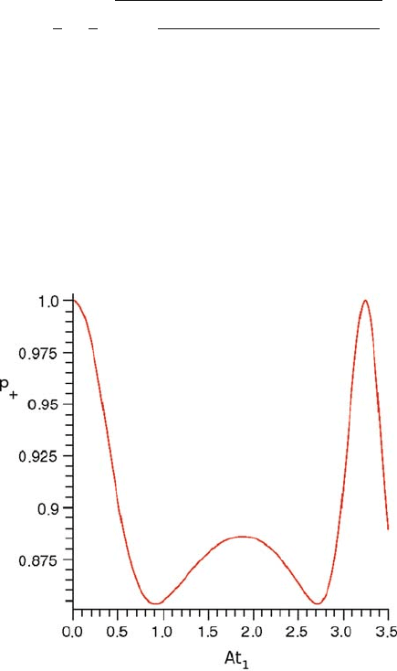
Fig. 6.9 (Color online) The eigenvalue p
+
of the reset matrix right after the first photon at time t
1
,
as a function of t
1
, for the same initial state and parameters as in Fig. 6.8. In the center of the time
interval, p
+
differs appreciatively from 1 and thus ˆρ considerably deviates from a pure state
In Fig. 6.9 we have plotted p
+
as a function of the time t
1
of the first photon,
for the same initial state and parameters as in Fig. 6.8. At the initial time one has
the initial pure state and hence p
+
= 1. Whenever p
+
< 1, ˆρ is a mixture, and the
deviation from a pure state is the more pronounced the closer p
+
is to 1/2.
Figure 6.10 shows that the eigenvectors of the reset matrix ˆρ can deviate signif-
icantly from |1 and |2. In this figure we have plotted the absolute value, R,ofthe
ratio of the first and second components of |p
+
as a function of the time t
1
of the
first photon, for the same initial state and parameters as in Fig. 6.8. In the center
of the depicted time interval the first and second components of |p
+
are of similar
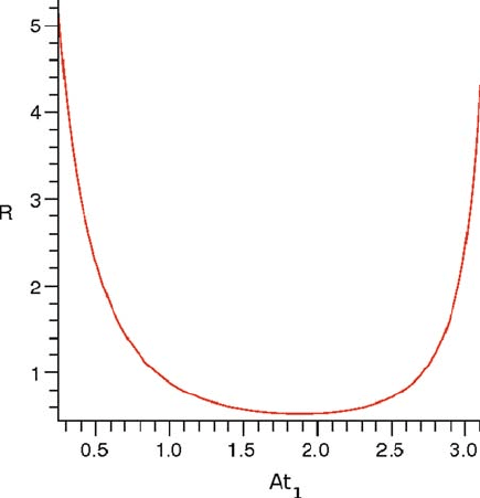
6 The Quantum Jump Approach and Some of Its Applications 159
Fig. 6.10 (Color online) Absolute value, R, of the ratio of the first and second components of the
eigenvector |p
+
of the reset matrix, as a function of the time t
1
, for the same initial state and
parameters as in Fig. 6.8. In the center of the time interval the first and second components of |p
+
are of similar magnitude, while at the boundary times it is predominantly in |1
magnitude, while at times close to the boundary of the figure |p
+
is close to |1and
|p
−
close to |2.
For a simulation one now has two quite different situations. When one starts in
the atomic state |1, the atom is pumped to a superposition of |3 and |1.Afterthe
first photon it jumps to |2. After the second photon it jumps from |2 to |1,so
after two photons one is back to the original starting state |1 and the simulation
continues as before. When one starts in the atomic state |2, the atom decays to |1,
and after that the simulation continues as before.
However, if one starts from a superposition of |1and |2, which can be prepared,
e.g., by a pulse from a second laser, the situation is completely different. In this case
the atom will in general be reset to a nonpure state right after the first photon. In
a simulation one would then have to continue the conditional time development
until the next photon with a density matrix. For a higher dimensional atomic state
space a simulation with density matrices is much more time consuming than with
pure states. As noted at the beginning of this section, one can bypass this compli-
cation and go over to a sequence of (simulated) pure states, without changing the
overall jump statistics in a trajectory and still generating the Bloch equations for an
ensemble of such trajectories [26]. This tremendously reduces numerical effort in
more complicated cases. We will demonstrate this procedure in the simple cascade
160 G.C. Hegerfeldt
model outlined above, although in this case the numerical simplifications are not so
pronounced.
Replacing density matrices by pure states in simulations: Onestartsinthestate
|α, develops with U
cond
(t, 0), calculates the probability density w
1
(t, t
0
= 0; |α)
for the first photon as in (6.122), and generates the first photon time, t
1
, by a random
number generator according to this probability density. Then one determines the
corresponding reset matrix ˆρ ≡ ˆρ(t
1
) as in (6.123). Instead of resetting the atomic
state to ˆρ(t
1
) one determines its eigenvalues p
±
(t
1
) and eigenstates |p
±
(t
1
) and
resets the atom to the pure state |p
+
(t
1
) with probability p
+
(t
1
)orto|p
−
(t
1
) with
probability p
−
(t
1
). Then one applies the conditional time development U
cond
(t, t
1
)
to the pure state chosen and calculates the probability density w
1
(t, t
1
; |p
±
(t
1
))for
the second photon. With this probability density one generates the time, t
2
, for this
second photon and determines the reset matrix at time t
2
, which obviously depends
on the pure reset state chosen at time t
1
. Again, instead of resetting the atom to this
reset matrix, one resets to one of its eigenvectors with the probability given by the
corresponding eigenvalue. This procedure is depicted in Fig. 6.11. Continuing in
this way, one generates a pseudo-quantum trajectory with pure states which does
not correspond to an actual physical trajectory. Nevertheless, the jump statistics
obtained by time averaging over such a trajectory agrees with the photon statistics
of the original physical process [26].
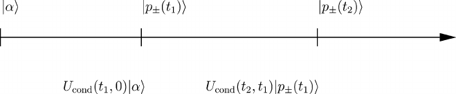
Fig. 6.11 Simulation of a trajectory consisting of pure states. One starts in |α, develops with U
cond
,
generates the first jump time t
1
, and determines the reset state for U
cond
(t
1
, 0)|αand its eigenvalues
p
±
(t
1
) and eigenvectors |p
±
(t
1
).Att
1
one resets to |p
±
(t
1
) with probability p
±
(t
1
). Then one
develops the chosen reset state with U
cond
(t, t
1
), generates the next jump time t
2
, and determines
the reset state for U
cond
(t
2
, t
1
)|p
±
(t
1
) and its eigenvalues p
±
(t
2
) and eigenvectors |p
±
(t
2
).Att
2
one resets to |p
±
(t
2
) with probability p
±
(t
2
),andsoon
Recovering the Bloch equations: Now one can repeatedly generate a large ensem-
ble of such trajectories, always starting with the same initial state |α. At a fixed time
t, each trajectory is in a particular pure state, which depends on its history. Let the
incoherent weighted sum of these states be denoted by ρ
(sim)
|α
(t). It can then be shown
[26] that this density matrix satisfies the optical Bloch equations of the original
problem with the same initial condition, i.e., |αα|, and hence renders a solution of
the Bloch equations of the original problem. In general, for a large number of levels,
this can be numerically extremely advantageous.

6 The Quantum Jump Approach and Some of Its Applications 161
6.7 Inclusion of Center-of-Mass Motion and Recoil
6.7.1 Conditional Hamiltonian and Reset Operation
Until now, the N-level system was assumed to be at rest. For atoms or ions in a trap
this is often a good approximation. In general, however, the motion of the system
should be taken into account, in particular when the laser intensity varies in space
and when the center-of-mass (cm) motion should be treated quantum mechanically,
as for lower velocities.
As an example we consider a two-level system with quantized cm motion, inter-
acting with a classical laser and with the quantized radiation field. In the Schr
¨
odinger
picture the corresponding Hamiltonian is of the form
H =
ˆ
P/2m +ω
0
|22|+
ω
k
a
†
kλ
a
kλ
+e
ˆ
D ·E(
ˆ
X, 0) +e
ˆ
D ·E
L
(
ˆ
X, t) , (6.131)
where
ˆ
X and
ˆ
P denote cm position and momentum operator and
ˆ
D the dipole oper-
ator as in (6.11). The classical laser field is of the form
E
L
(x, t) = Re E
0
(x)e
−iω
L
t
, (6.132)
where we allow for a position-dependent laser amplitude. We put
g
kλ
≡ ie
ω
k
2ε
o
V
ε
kλ
·D
12
and go over to a “laser-adapted cm field interaction picture” by means of the
operator
˜
H
0
L
=
ˆ
P
2
/2m + ω
L
|22|+H
0
F
(6.133)
and denote the resulting Hamiltonian by H
Lcm
I
. With the rotating wave approxima-
tion one then has in this interaction picture
H
Lcm
I
=−Δ|22|
+|12|
g
kλ
a
k,λ
exp{−i(ω
k
−ω
L
)t}exp{ik · (
ˆ
X +
ˆ
Pt/m)}+h.c.
+
2
|21|Ω(
ˆ
X +
ˆ
Pt/m) +h.c., (6.134)
where Δ = ω
L
−ω
0
is the detuning and the position-dependent Rabi frequency is
Ω(x) = eD
12
·E
0
(x) .
As is (6.7) we consider the zero-photon matrix element of the time-development
operator from t to t +Δt. In the Dyson series of the time-development operator we

162 G.C. Hegerfeldt
keep only terms proportional to Δt. Then only the laser contributes to the first order,
which is
−
i
t+Δt
t
dt
,
2
|21|Ω(
ˆ
X +
ˆ
Pt
/m) +h.c.
-
.
The second-order term in the time-development operator becomes
−
i
2
0
ph
|
t+Δt
t
dt
t
t
dt
H
Lcm
I
(t
)H
Lcm
I
(t
) |0
ph
=
−
1
2
|22|
t+Δt
t
dt
t
t
dt
kλ
|g
kλ
|
2
exp{i(ω
k
−ω
L
)(t
−t
)}
exp{ik ·(
ˆ
X +
ˆ
Pt
/m)}exp{−ik ·(
ˆ
X +
ˆ
Pt
/m)} , (6.135)
where again, as in Sect. 6.2.1, the laser terms have been omitted since they are
proportional to (Δt)
2
.
We note that
ˆ
X(t
) ≡
ˆ
X +
ˆ
Pt
/m =
ˆ
X +
ˆ
Pt/m +
ˆ
P(t
−t)
is the time development of
ˆ
X in the free Heisenberg picture of the cm motion of the
system. With Δt ≈ 10
−12
s as in (6.1) and the atomic velocity around 1 m/s one has
Δx ≡ νΔt = 10
−12
m. With optical wavelengths one has k ∼ 2 ×10
6
m
−1
so that
kΔx ∼ 2 ×10
−6
and therefore the
ˆ
P(t
− t) part can be neglected in the exponent.
It can similarly be neglected in Ω(
ˆ
X +
ˆ
Pt
/m) of the first-order term if Ω(x) does
not vary significantly over a distance of Δx. Hence, under these conditions one has
ˆ
X(t
) ≈
ˆ
X(t
) ≈
ˆ
X(t) . (6.136)
Then the last two exponentials in (6.135) cancel. As in Sect. 6.2.1 for the two-
level case without cm motion this leads to the damping term −
1
2
A|22| and one
obtains as conditional Hamiltonian in the laser-adapted cm interaction picture
H
Lcm
cond
=−Δ|22|−
i
2
A|22|+
2
Ω(
ˆ
X(t))|21|+h.c.. (6.137)
Reversing the interaction picture with respect to the free cm Hamiltonian, one
obtains for the conditional Hamiltonian in the laser-adapted interaction picture,
denoted as in (6.36) by H
IL
cond
,
H
IL
cond
=
ˆ
P
2
/2m − Δ|22|−
i
2
A|22|+
2
Ω(
ˆ
X)|21|+h.c.. (6.138)
In the Schr
¨
odinger picture this becomes