Muga G. Time in Quantum Mechanics - Vol. 2
Подождите немного. Документ загружается.

6 The Quantum Jump Approach and Some of Its Applications 133
H
0
A
= ω
0
|
22
|
, H
0
F
=
kλ
ω
k
a
†
kλ
a
kλ
, (6.13)
ˆ
D
(−)
= D
21
|21| , D
ij
=i|X|j , (6.14)
ˆ
E
(+)
=
kλ
ie
ω
k
2ε
0
V
1/2
ε
kλ
a
kλ
,
E
(+)
ext
(t) =
1
√
2π
∞
0
dω
˜
E
ext
(ω)e
−iωt
,
and a frequency cutoff is included. V is the quantization volume, later taken to
infinity, a
†
kλ
and a
kλ
are the photon creation and annihilation operators, and ε
kλ
a
polarization vector. For an external laser field of frequency ω
L
,
E
L
(t) = Re E
0
e
−iω
L
t
, (6.15)
and the Rabi frequency, Ω, is defined as
Ω = eD
12
·E
0
. (6.16)
For an external laser field, H
AL
(t) then becomes, in the rotating-wave approxima-
tion,
H
AL
(t) =
Ω
2
|21|e
−iω
L
t
+h.c.
, (6.17)
where the Rabi frequency Ω plays the role of a coupling constant.
Going over to the interaction picture with respect to H
0
A
+ H
0
F
one has
H
I
(t) = H
I
AL
(t) + H
I
AF
(t) , (6.18)
which is obtained by replacing |21|and a
kλ
in the original interaction Hamiltonian
by |21|e
iω
0
t
and a
kλ
e
−iω
k
t
, respectively. We now calculate, for t
i
≤ t
< t
i+1
,
0
ph
|
d
dt
U
I
(t
, t
i
) |0
ph
. (6.19)
In the first-order contribution only H
I
AL
(t) remains since H
I
AF
(t) is linear in the
creation and annihilation operators and hence
0
ph
|H
I
AF
(t)|0
ph
=0 . (6.20)
The second-order contribution is, by (6.20),
−
−2
t
t
i
dt
0
ph
|H
I
AF
(t
)H
I
AF
(t
)|0
ph
+H
I
AL
(t
)H
I
AL
(t
)
. (6.21)

134 G.C. Hegerfeldt
Now, if the external field E
ext
(t) is smooth in time, e.g., given by laser, and not
wildly fluctuating like a thermal or chaotic field, then the second part in (6.21) con-
tributes a term of higher order in Δt and can therefore be omitted. For a chaotic
external field, however, this part may give rise to a contribution of the order of Δt
and then has to be retained. In this case one can no longer work with state vectors
(wavefunctions) but has to use (conditional) density matrices. A particular example
of this is treated in [30].
Thus, supposing a smooth external field, only terms of the form aa
†
survive in
the second-order contribution, which then becomes
−
−2
t
t
i
dt
|21|12|
kλ
e
2
ω
k
2ε
0
V
(D
21
·ε
kλ
)(ε
kλ
·D
12
)e
−i(ω
k
−ω
0
)(t
−t
)
=−
−2
|22|
t
−t
i
0
dτ
kλ
e
2
ω
k
2ε
0
V
(D
21
·ε
kλ
)(ε
kλ
·D
12
)e
−i(ω
k
−ω
0
)τ
. (6.22)
One can now use properties of the correlation function
κ(τ ) ≡
kλ
e
2
ω
k
2ε
0
V
(D
21
·ε
kλ
)(ε
kλ
·D
12
)e
−i(ω
k
−ω
0
)τ
. (6.23)
With V
−1
= Δ
3
k/(2π)
3
one can perform the limit V →∞, and the sum over k
becomes an integral over ω, with a suitable frequency cutoff, and an integral over
the unit sphere. The correlation function has an effective width of the order of ω
−1
0
around τ = 0, and for t
− t
i
ω
−1
0
one can therefore extend the τ integration in
(6.22) to infinity [2]. This amounts to the replacement
t
−t
i
0
dτ e
i(ω
0
−ω
k
)τ
∼
=
πδ(ω
k
−ω
0
) + iP
1
ω
k
−ω
0
(6.24)
and corresponds to the usual Markov approximation in the derivation of the optical
Bloch equations [38, 43]. The principal-value term is analogous to a level shift and
will be omitted [16, 43]. For the second-order contribution one then obtains
−|22|
d
3
k
e
2
ω
k
(2π)
3
2
0
D
21
·
2
λ=1
ε
kλ
ε
kλ
·D
12
πδ(ω
k
−ω
0
) . (6.25)
The last integral is denoted by Γ and using
2
λ=1
|ε
kλ
·D
12
|
2
=|D
12
|
2
−|
ˆ
k · D
12
|
2
(6.26)
one obtains

6 The Quantum Jump Approach and Some of Its Applications 135
Γ ≡
e
2
6πε
0
c
3
|D
21
|
2
|ω
0
|
3
= A/2 , (6.27)
where A is the usual Einstein coefficient.
Hence, integrating over t
from t
i
to t
i+1
and using 1 + α ≈ e
α
for small α,we
obtain
0
ph
|U
I
(t
i+1
, t
i
)|0
ph
=exp
−
i
t
i+1
t
i
dt
H
I
AL
(t
) −iΓ |22|
. (6.28)
For small Δt this can be replaced by a time-ordered exponential,
0
ph
|U
I
(t
i+1
, t
i
)|0
ph
=T exp
−
i
t
i+1
t
i
dt
H
I
AL
(t
) −iΓ |22|
≡U
I
cond
(t
i
, t
i−1
) .
(6.29)
From this, one has, with t = t
n
,
n
4
i=1
0
ph
|(U
I
(t
i
, t
i−1
)|0
ph
=T exp
−
i
t
0
dt
H
I
AL
(t
) − iΓ |22|
=U
I
cond
(t, 0) ,
(6.30)
where the product sign on the l.h.s. includes an ordering in an obvious way.
Since
0
ph
|U(t
i
, t
i−1
)|0
ph
=e
−iH
0
A
t
i
/
0
ph
|U
I
(t
i
, t
i−1
)|0
ph
e
iH
0
A
t
i−1
/
(6.31)
and since, for t = t
n
= nΔt,
U
cond
(t, 0) =
n
4
i=1
0
ph
|U(t
i
, t
i−1
)|0
ph
,
we obtain, on a coarse-grained timescale, from (6.30) and (6.31)
U
cond
(t, 0) = T exp
−
i
t
0
dt
H
0
A
+ H
AL
(t
) − iΓ |22|
, (6.32)
which is the transformation of (6.30) back to the Schr
¨
odinger picture.
Thus the conditional Hamiltonian for a two-level atom with no photon emission
until time t is given, on the coarse-grained timescale, by
H
cond
(t) = H
0
A
+ H
AL
(t) −i
A
2
|22| . (6.33)

136 G.C. Hegerfeldt
It may be worthwhile to point out that (6.29) can be derived directly in a more
elaborate way without recourse to perturbation theory by means of the Markov prop-
erty alone. Therefore the possible errors involved in going from (6.19) to (6.29) do
not add up.
6.2.2 First-Photon Probability Density for a Laser-Driven
Two-Level System
For an external laser field one has
H
cond
(t) = ω
0
|
22
|
+
Ω
2
|21|e
−iω
L
t
+h.c.
−i
A
2
|22| . (6.34)
It is noteworthy that one can get rid of the time dependence by going over to a
“laser-adapted interaction picture” by means of the operator
H
0
L
= ω
L
|22| (6.35)
instead of H
0
A
. In this interaction picture the conditional Hamiltonian becomes
H
IL
cond
=−Δ
|
22
|
+
Ω
2
{
|21|+|12|
}
−i
A
2
|22| , (6.36)
where Δ = ω
L
−ω
0
is the detuning. In matrix form this reads
H
IL
cond
/ =
0 Ω/2
Ω/2 −Δ −iA/2
. (6.37)
In these expressions one clearly sees that the imaginary term leads to a decrease of
the state vector norm – this corresponds to a decrease of the probability P
0
(t)of
finding no photon until time t.
From (6.6) one then obtains for the probability density for the first photon
w(t) =−
d
dt
P
0
(t)
=−
d
dt
||exp{−iH
cond
t/}|ψ
A
(0)||
2
=
i
ψ
cond
(t)|H
cond
− H
†
cond
|ψ
cond
(t) .
(6.38)
For the two-level system this becomes
w(t) = A |2|exp{−iH
IL
cond
t/}|ψ
A
(0)|
2
. (6.39)
6 The Quantum Jump Approach and Some of Its Applications 137
If λ
±
denote the eigenvalues of H
IL
cond
/ then the conditional time-development
operator in this interaction picture is given by
exp{−iH
IL
cond
t/}=
1
λ
+
−λ
−
e
−iλ
+
t
1
H
IL
cond
−λ
−
2
−e
−iλ
−
t
1
H
IL
cond
−λ
+
2
.
(6.40)
This identity can be checked directly by applying both sides of the equation to
the eigenvectors |λ
±
. If one starts in the atomic ground state, |ψ
A
(0)=|1, one
obtains for ω
L
= ω
0
(zero detuning, Δ = 0)
λ
±
=−
iA
4
±
1
4
/
4Ω
2
− A
2
,
(6.41)
and for the first-photon probability density
w(t) =
4AΩ
2
|4Ω
2
− A
2
|
e
−At/2
sin
1
4
/
4Ω
2
− A
2
t
2
.
(6.42)
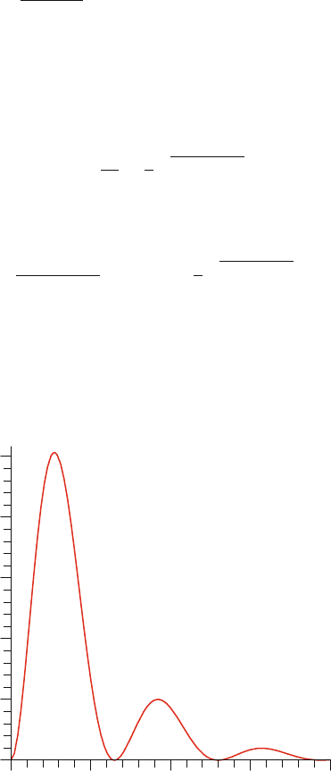
This probability density is plotted in Fig. 6.5 for Ω = 2A. It should be noted that
w(0) = 0. This is connected to the so-called anti-bunching of photons as follows.
One can imagine that at time t = 0 a photon was emitted, right after which the
atom is in the ground state. Hence w(0) = 0 means that in light emitted from the
w/A
At
0.4
0.3
0.2
0.5
0.1
0.0
2.5 10.05.0 7.50.0
Fig. 6.5 (Color online) Probability density, w(t), for the first photon as a function of time for a
laser-driven two-level system, with Ω = 2A. The vanishing of w(t)fort = 0 implies anti-bunching
of photons

138 G.C. Hegerfeldt
atom there is only a small probability to find two photons in quick succession. This
is in contrast to natural (chaotic) light where there is bunching, i.e., photons tend
to come in pairs. Anti-bunching, which is usually derived by means of the optical
Bloch equations, just reflects the fact that it takes some time for the light source to
pump the atom back to the excited state before the next photon can be emitted.
From (6.42) the mean waiting time, τ , for the first photon is calculated as
τ =
2Ω
2
+ A
2
AΩ
2
. (6.43)
This result will be used later in connection with the discussion of macroscopic light
and dark periods.
6.2.3 Connection with the Quantum Zeno Effect
When one lets Δt become smaller and smaller the above derivation shows very
nicely how and where the quantum Zeno effect [39] turns up in a very natural way. If
Δt is chosen much smaller than the inverse optical frequencies, the last exponential
in (6.22) can be replaced by 1, and the integral becomes proportional to t
− t
i
.
Equation (6.28) is then replaced by
0
ph
|U
I
(t
i+1
, t
i
)|0
ph
=exp
−
i
H
AL
(t
i
)Δt −i const |22|(Δt)
2
. (6.44)
The time-ordered product of these operators then becomes, for Δt → 0,
T exp
−
i
t
0
dt
H
I
AL
(t
)
. (6.45)
This is a purely atomic operator, and hence the time development of the field
becomes frozen, i.e., for Δt → 0 one always remains in the vacuum and the tem-
poral change occurs only in the atomic subspace. For this reason one cannot choose
Δt arbitrarily small in the quantum jump approach.
6.2.4 Jumps and Reset Operation
With the detection of a photon the conditional time development terminates and the
atom “jumps” to a new state. For a two-level system it is intuitively clear that right
after a photon detection the atom should be in its ground state and it would seem to
use overkill to calculate this by the general more involved theory. It is instructive,
however, to see how the machinery works for this simple system and it clarifies the
procedure for the general case.

6 The Quantum Jump Approach and Some of Its Applications 139
We consider an ensemble where no photons are present at some time t.Atthis
instant the total ensemble is thus described by a state |0
ph
|φ or more generally by
a density matrix ρ
tot
(t) =|0
ph
ρ0
ph
| where ρ is the density matrix of the atoms.
The (normalized) state of the subensemble for which photons are detected by a
nonabsorptive measurement at time t + Δt is given, in view of the von Neumann–
L
¨
uders projection postulate [1], by
P
1
ρ
tot
(t +Δt)P
1
/tr(·) , (6.46)
where
P
1
≡ 1 −|0
ph
1
A
0
ph
| , (6.47)
and where the trace of P
1
ρ
tot
(t +Δt)P
1
gives the probability of detecting a photon
in the time interval Δt. Note that (6.46) still contains the photons.
After a photon measurement by absorption no photons are present any longer and
it was argued in [23] that the resulting state is obtained from (6.46) by a partial trace
over the photons, i.e., by
|0
ph
tr
ph
P
1
ρ
tot
(t +Δt)P
1
0
ph
|/tr(·) . (6.48)
The physical reason for this is that for the atomic description alone it should make
no difference in infinite space whether or not the photons are absorbed, as long as
they are sufficiently far away from the atom and no longer interacting with it.
2
We
define the superoperator R, which acts on atomic density matrices, by
RρΔt ≡ tr
ph
P
1
U(t + Δt, t)|0
ph
ρ 0
ph
|U
†
(t +Δt, t)P
1
(6.49)
and call R the reset operation and Rρ/tr(·) the (normalized) reset state. The atomic
trace of RρΔt gives the probability of detecting a photon in the time interval Δt
when initially there were no photons and the atom was in the state ρ.
Equation (6.49) can be calculated by perturbation theory for U
I
(t +Δt, t), as in
Sect. 6.2.1. Now the first-order contribution suffices and in this order the external
(laser) field drops out since P
1
|0
ph
=0. One obtains in a straightforward way
RρΔt =e
−iH
0
A
Δt/
|12|ρ|21|e
iH
0
A
Δt/
×
Δt
0
dt
Δt
0
dt
kλ
e
i(ω
k
−ω
0
)(t
−t
)
e
2
ω
k
2ε
0
V
(D
12
·ε
kλ
)(ε
kλ
·D
21
) .
(6.50)
To apply the Markov property, we decompose the rectangular integration domain
over t
and t
in (6.50) into two triangles, leading to
2
For a cavity, however, where photons can return and revivals can occur, the results are different.
140 G.C. Hegerfeldt
Δt
0
dt
t
0
dt
e
i(ω
k
−ω
)
(t
−t
)
+
Δt
0
dt
t
0
dt
e
i(ω
k
−ω
)
(t
−t
)
.
(6.51)
As in (6.22) and (6.24), by the properties of the correlation function, each of the
inner integrals can be replaced by πδ(ω
k
− ω
0
) where the principal values cancel
each other. In this way one obtains
RρΔt = A|12|ρ|21|Δt
= Aρ
22
|11|Δt .
(6.52)
Thus, as expected, the probability density is given by the Einstein coefficient multi-
plied by the occupation of the excited level, and after detection of a photon the atom
is in the ground state. The appearance of the Einstein coefficient and the ground
state reflects the fact that one observes spontaneous photons only since the laser is
treated classically. Anyway, if the laser photons were treated quantum mechanically
it should be recalled that photons from stimulated emissions have the same direction
as the incident, stimulating, laser photons and are therefore not observed.
Now, if instead of a normalized atomic density matrix one takes the conditionally
time-developed state |ψ
cond
(t), then the atomic trace of
R
(
|ψ
cond
(t)ψ
cond
(t)|
)
(6.53)
gives the probability density for a photon at time t under the condition that no photon
has been detected before, i.e., the probability density for the first photon after t = 0.
This was denoted by w(t) in (6.42) and therefore
w(t) = tr
R
(
|ψ
cond
(t)ψ
cond
(t)|
)
.
(6.54)
The general reset state for systems at rest has been determined in [23, 34] and is
given in Sect. 6.4. It may depend on |ψ
cond
(t
1
) where t
1
is the detection time of the
photon.
6.2.5 Quantum Trajectories
One can now distinguish different steps in the temporal behavior of the single atom
under the above gedanken measurements.
(i) Until the detection of the first photon, the atom belongs to the subensembles
E
(nΔt)
0
and hence is described by the (non-normalized) vector
|ψ
cond
(t)=U
cond
(t, 0)|ψ
A
(0) . (6.55)

6 The Quantum Jump Approach and Some of Its Applications 141
(ii) The first photon is detected at some (random) time t
1
, according to the proba-
bility density
w(t) =−
dP
0
(t)
dt
=−
d
dt
|ψ
cond
(t)
2
. (6.56)
(iii) Jump: With the detection of a photon the atom has to be reset to the appropriate
state. For example, a two-level atom will be in its ground state right after a
photon detection.
(iv) From this reset state the time development then continues with U
cond
(t, t
1
),
until the detection of the next photon at the (random) time t
2
. Then one has to
reset (jump), and so on.
In this way one obtains a stochastic path in the Hilbert space of the atom. The
stochasticity of this path is governed by quantum theory, and the path is called a
quantum trajectory. In general the reset state will not be a pure state but a density
matrix, as explained in Sect. 6.4.2, and this may result in quantum trajectories with
density matrices instead of pure states, even if one starts in a pure state. However,
it is pointed out in Sect. 6.6 that one can replace such a trajectory by a trajectory
consisting of pure states only. The stochastic process underlying the quantum tra-
jectories is a jump process with values in a Hilbert space. If the reset state is always
the same, e.g., the ground state, one has a renewal process. If the reset state depends
on the conditional state before the jump, one has a Markov process only.
In which sense the parts of a trajectory between jumps can be regarded as an
ensemble created by repetition from a single system at stochastic times will be
discussed in the last section.
The steps (i)–(iv) above can be used for simulations of a trajectory. This will be
discussed in more detail in Sect. 6.6 for the specific example of a three-level cascade
system.
6.3 Application: Macroscopic Light and Dark Periods
The ideas of the preceding section will now be used to provide a direct quantum
mechanical understanding of macroscopic light and dark periods without employing
Bloch equations or a rate-equation approach. For the V system of Fig. 6.1 which
employs two coherent light sources the QJA as described so far can be applied right
away. For setups which in addition to a laser also have driving by a lamp the QJA
has to be carried over to include incoherent driving. This has been done in [30],
and those results can be used to discuss those experimentally realized systems in
[10–13] which have driving by a lamp.
In this section the QJA will be applied to the V system of Fig. 6.1. A strong
laser of frequency ω
L1
drives the 1–2 transition, while the transition from 1 to the
metastable state 3 is weakly driven by a laser of frequency ω
L2
. It is assumed that
the laser frequencies are close to the transition frequencies ω
2
and ω
3
and that the

142 G.C. Hegerfeldt
latter are far apart. Then instead of (6.12), (6.13), and (6.17) one has
H
0
A
=ω
2
|22|+ω
3
|33| ,
D
i1
=i|X|1 ,
ˆ
D
(−)
= D
21
|21|+D
31
|31| ,
H
AL
(t) =
Ω
1
2
|21|e
−iω
L1
t
+h.c.
+
Ω
2
2
|31|e
−iω
L2
t
+h.c.
,
(6.57)
where Ω
1
and Ω
2
are the respective Rabi frequencies characterizing the strength of
the atom–laser interaction. One can now determine the conditional Hamiltonian for
this system either as in the preceding section or by using the general expression in
(6.83). Written in an obvious matrix form the result is of the form
H
cond
/ =
⎛
⎝
0e
iω
L1
t
Ω
1
/2e
iω
L2
t
Ω
2
/2
e
−iω
L1
t
Ω
1
/2 ω
2
−iA
2
/2 −iγ
12
e
−iω
L2
t
Ω
2
/2 −iγ
21
ω
3
−iA
3
/2
⎞
⎠
, (6.58)
where A
2
and A
3
are the respective Einstein coefficients and where the γ
ij
terms
will later be seen to be negligible by the rotating-wave approximation. Going over
to a “laser-adapted interaction picture” by means of the operator
H
0
L
= ω
L1
|22|+ω
L2
|33|, (6.59)
one obtains, with the detunings Δ
1
= ω
L1
−ω
2
and Δ
2
= ω
L2
−ω
3
,
H
IL
cond
/ =
⎛
⎝
0 Ω
1
/2 Ω
2
/2
Ω
1
/2 Δ
1
−iA
2
/20
Ω
2
/20Δ
2
−iA
3
/2
⎞
⎠
, (6.60)
where the rapidly oscillating terms γ
ij
exp{±i(ω
L2
−ω
L1
)t} can be, and have been,
omitted. It will be assumed in the following that
Ω
2
1
Ω
2
2
, A
3
A
2
and A
2
A
3
,Ω
2
(6.61)
as well as Δ
1
= 0. From the inequalities it follows that the upper left 2 × 2matrix
dominates. (This becomes evident if one adds Δ
2
1 to H
IL
cond
/ to get rid of −Δ
2
in the 33 component of the matrix.) The upper left 2 × 2 matrix is the same as in
(6.37) for a two-level system. Therefore, two of the eigenvalues, λ
1,2
,ofH
IL
cond
/ are
approximately given by (6.41) and the third by
λ
3
+Δ
2
∼−iA
3
. (6.62)
Therefore, there are different orders of magnitudes present in the imaginary parts of
the eigenvalues and one has
−Imλ
3
−Imλ
1,2
. (6.63)