Muga G. Time in Quantum Mechanics

Подождите немного. Документ загружается.

6 The Quantum Jump Approach and Some of Its Applications 163

cond

/2m + ω

|22|−

A|22|+



Ω(

X)|21|e

−iω

+h.c.,

(6.139)

which is the analog of (6.34).

The reset operation looks somewhat different if cm motion is included. The

atomic density operator ρ now describes both the cm motion and the internal two-

level degrees of freedom. Therefore, if one takes matrix elements with momentum

eigenvectors of the cm motion, then

ρ(p, p



) ≡p|ρ|p



 (6.140)

becomes an operator for the internal degrees of freedom, which corresponds to a

2 × 2 matrix in case of a two-level system. The reset operation R is again given

by the general expression in (6.49), but now with the Hamiltonian from (6.131). As

before, in ﬁrst-order perturbation theory the external ﬁeld drops out and one obtains

instead of (6.50)

RρΔt =



Δt





Δt





kλ

i(ω

−ω

)(t



−t



)

2ε

V

|ε

kλ

·D

−ik·

X(t



)

|12|ρ|21|e

ik·

X(t



)

(6.141)

Similarly as before one can replace

X(t



) and

X(t



)by

X, by (6.136). Note that since

2|ρ|2 is a cm operator, it does not commute with

X. Now one can proceed as in

(6.51) to split the double integral and use the property of the correlation function.

Again this gives a πδ(ω

−ω

) which allows to perform the k

dk integration. This

gives

Rρ = A|11|



dΩ

−|

k · D

−ik·

2|ρ|2e

ik·

(6.142)

where the angular integration is over the unit vectors

k. In momentum space one has

ik·

|p=|p + k (6.143)

and this gives with (6.142)

p|Rρ|p



=A|11|



dΩ

1 −

k · D

2|p + ω

k/c| ρ |p



+ω

k/c|2 .

(6.144)

The ﬁrst factor in the integral is the usual dipole emission characteristics and the

terms ω

k/c yield momentum conservation after the photon emission. We note

164 G.C. Hegerfeldt

that the resulting reset matrix is a pure state only for internal degrees of freedom but

not for the cm variables, even if the density matrix before the photon detection is a

pure state.

Instead of asking for the detection of any photon one may ask for a photon detec-

tion in a given direction

k. Then the reset operation, R

, is given by

p|R

ρ|p



=A|11|(1 −

k · D|

)2|p + ω

k/c| ρ |p



+ω

k/c|2 ,

(6.145)

which reﬂects the dipole emission characteristics. If ρ is a pure state in momentum

space this is again a pure state. The probability to detect a photon with direction in

the solid angle dΩ

in the time interval dt is given by

tr R

ρ dΩ

dt . (6.146)

Integrating (6.145) over all directions gives the reset matrix in (6.144).

Similarly, one may ask for a photon detection in a given direction

k and given

polarization λ. The corresponding reset operation, R

kλ

, is then given by

p|R

ρ|p



=A|11|

|ε

kλ

·D

2|p + ω

k/c| ρ |p



+ω

k/c|2 .

(6.147)

Again, if ρ is a pure state in momentum space this is again a pure state, and the

analog of (6.146) holds.

In simulations of quantum trajectories of a two-level system with cm one can

work with the reset operation R

or with R

and thus with pure states when one

starts in a pure state [45]. In this case one does not need the more complicated

procedure of Sect. 6.6.

6.7.2 Application to Quantum Arrival Times

An important open problem in quantum theory is the question of how to formulate

the notion of “arrival time” of a particle, such as an atom, at a given location, i.e., the

time instant of its ﬁrst detection there. This is clearly a very physical question, but

when the extension and spreading of the wave packet is taken into account, a satis-

factory formulation is far from obvious. The problem of time in quantum mechanics,

both for time instants and time durations such as dwell time, has received a great

deal of theoretical attention recently [40]. When the translational motion of the par-

ticle can be treated classically, a full quantum analysis of arrival time is in fact not

necessary. This is the case for fast particles, and therefore arrival times are presently

measured mostly by means of time-of-ﬂight techniques, whose analysis is carried

6 The Quantum Jump Approach and Some of Its Applications 165

out in terms of classical mechanics. Problems, though, arise for slow particles for

which the ﬁnite extent of the wavefunction and its spreading become relevant, such

as for cooled atoms dropping out of a trap. Then a quantum theoretical point of view

is needed. It is therefore important to ﬁnd out when the classical approximations

fail and to propose measurement procedures for arrival times in the quantum case.

Since the theoretical deﬁnition of a quantum arrival time is still subject to debate it

is necessary to determine what exactly such measurement procedures are measuring

and to compare such operational approaches with the existing, more abstract and

axiomatic, theories.

An experimentally very natural approach to determine the arrival time of an atom

is by quantum optical means. A region of space may be illuminated by a laser and

upon entering the region an atom will start emitting photons. The ﬁrst photon emis-

sion can be taken as a measure of the arrival time of the atom in that region.

It is easiest to ﬁrst study the 1D case and use the corresponding equations of Sect.

6.7.1. Then (6.139) simply becomes 1D in p and x. Illuminating the half axis x > 0

perpendicularly by a laser, the Rabi frequency Ω(x) becomes a multiple of the step

function Θ(x). In [18] the corresponding conditional time development has been

solved explicitly and the distribution of the ﬁrst-photon times have been calculated.

If one deducts by a deconvolution technique the delays due to the ﬁnite pumping

time, one obtains in the limit of weak pumping a surprising result for the arrival

time distribution, namely the usual well-known quantum mechanical probability

ﬂux. More details can be found in Chap. 4.

Another model for arrival times will be discussed in Sect. 6.8. This model couples

the center-of-mass motion to spins which in turn are coupled to bosons. The arrival

of the particle induces a spin ﬂip which in turn induces the emission of a boson.

6.8 Extension to Spin-Boson Models

In this section it will be shown in an example that the QJA can be extended to a

system which is coupled to a bath I which in turn is coupled to another bath, bath

II. Measurements are taken on bath II and from these one can infer properties of the

small system. Bath I serves as an ampliﬁer to enhance the signal and can be viewed

as a part of the measuring apparatus, a part which is treated quantum mechanically.

The model to be considered here consists of a moving particle coupled to a spatial

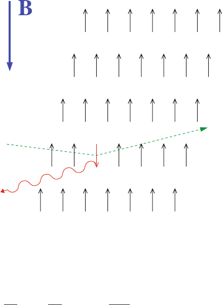
array of spins which in turn are coupled to bosons [21]. This model recently has been

used to study arrival times as well as passage times [27, 28]. In places where the par-

ticle wavefunction overlaps with a spin there is a high spin-ﬂip probability. Initially

the spins are in the (metastable) up state. When the particle passes a spin there is

a very high probability for a single spin ﬂip, accompanied by a boson emission, as

depicted in Fig. 6.12. The spin ﬂip leads to a large energetic gain for neighboring

spins and therefore to a large spin-ﬂip probability of the neighboring spins. By a

domino effect, this leads to a sudden ﬂip of all spins, accompanied by a burst of

bosons, which can be detected.

166 G.C. Hegerfeldt

Fig. 6.12 (Color online) Array of spins in a metastable state in a weak magnetic ﬁeld B. A passing

particle produces a single spin ﬂip, accompanied by a boson emission. By a domino effect, the spin

ﬂip causes all spins to ﬂip, accompanied by an avalanche of bosons

The Hamiltonian is taken as

H =



( j)

ˆσ

( j)

−



j< j



( jj



)

ˆσ

( j)

⊗ ˆσ

( jj



)

+





†



+



( j)

i f

( j)

†



ˆσ

( j)

−

+h.c.

+



( j)

(

)





( j)

i f

( j)

†



ˆσ

( j)

−

+h.c.

. (6.148)

The individual terms are the free Hamiltonian for the particle, the spin Hamiltonian

with ferromagnetic interaction, the free boson Hamiltonian, a small permanent spin-

bath coupling which induces very rare spontaneous spin ﬂips, and a further spin-bath

coupling which is strongly enhanced if the particle is close to a spin, i.e., |g

( j)

|

|γ

( j)

|, where χ

( j)

(x) is a sensitivity function, e.g., equal to 1 in a neighborhood of

the jth spin, while e

i f

( j)

are possible phase factors which will later be put to 1.

It should be noted that the Hamiltonian conserves the excitation number, which

is the sum of up spins and bosons. Hence a boson detection indicates a spin ﬂip,

which in turn indicates that the particle has passed close to a spin (unless one has an

extremely rare exceptional spontaneous spin ﬂip). Therefore, one can consider the

time of a boson detection as a signal for the arrival of the particle at the spin array so

that this model can be regarded as a model for arrival times [27, 28]. The motivation

6 The Quantum Jump Approach and Some of Its Applications 167

for this model comes from the desire to minimize the backreaction of the detection

on the particle by employing the intermediary spin system.

To illustrate how the QJA works for this model we use a simple example in one

space dimension, with a single spin and N discrete boson modes, where later N is

taken to inﬁnity. The modes ω



and coupling constants g



are taken as



= ω

n/N, n = 1, ···, N ,



=−iG



/N , (6.149)

where ω

is the maximal boson frequency. The particle wave packet is assumed

to come in from the left. The probability, P

disc

(t) (“disc” stands for “discrete”), of

ﬁnding the detector spin in state |↓at time t is given by

disc

(t) =







∞

−∞

|

x ↓ 1



|

(6.150)

≡ 1 − P

disc

(t) .

As long as no recurrences occur (i.e., no transitions |↓ 1



 →|↑ 0) one can

regard

disc

(t) =

disc

(t) =−

disc

(t) (6.151)

as the probability density for a spin ﬂip (i.e., for a detection) at time t.In

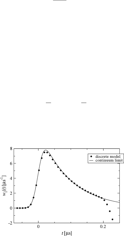
Fig. 6.13 the dots represent results of a numerical calculation of the spin-ﬂip prob-

ability density of N = 40 spins, for a sensitivity function χ(x) = Θ(x) and for

Fig. 6.13 Dots: spin-ﬂip probability density for incoming Gaussian wavefunction, N = 40,

χ(x) = Θ(x), where Θ is the step function; solid line: QJA result for continuum limit (N →∞),

the numerical evaluation is much faster

168 G.C. Hegerfeldt

an incoming Gaussian wavefunction. Numerically the calculation is extremely time

consuming.

Quantum jump approach: In the continuum limit, N →∞, the QJA can be

employed and leads to signiﬁcant numerical simpliﬁcations if the coupling constants

are such that the Markov property holds. This means here that for the correlation

function κ(τ ), now deﬁned as

κ(τ ) ≡





−i(ω



−ω

)τ

, (6.152)

there is a small correlation time τ

such that

κ(τ ) ≈ 0ifτ>τ

Then one can deﬁne A and δ

shift

, the analogs of Einstein coefﬁcient and level shift,

A ≡2Re



∞

dτκ(τ ) ,

shift

≡ 2Im



∞

dτκ(τ ) .

(6.153)

Proceeding as in Sect. 6.2, but now with Δt  τ

, one obtains that the time devel-

opment under the condition of no boson detection (i.e., no spin ﬂip) is given by the

conditional Hamiltonian

cond

/2m + /2(δ

shift

−iA)χ (

, (6.154)

where χ(x) is the sensitivity function. Formally, H

cond

is seen to contain a position-

dependent absorption and energy shift. The imaginary part leads to a decrease of the

wavefunction norm which physically means a decrease of the no-detection proba-

bility.

On a coarse-grained timescale one then ﬁnds, as in (6.38), for the probability

density of the ﬁrst boson (i.e., ﬁrst spin ﬂip)

(t) =−

(t)



ψ

cond

(t)|H

cond

− H

†

cond

|ψ

cond

(t)



dx χ(x)|x|ψ

cond

(t)|

(6.155)

If χ(x) is the characteristic function of an interval, where the spin is located, this is

just the decay rate A of the excited state of the detector multiplied by the probability

that the particle is inside the detector but is not yet detected – a very physical result.

6 The Quantum Jump Approach and Some of Its Applications 169

This result has been used to calculate w

(t), the solid curve in Fig. 6.13, for the

continuous version of (6.149), with χ (x) = Θ(x) and otherwise the same parame-

ters as for the discrete case. Up to the time of revivals – due to the discrete nature of

the bath – the agreement between the discrete version and the QJA result is excellent.

The numerical evaluation of the QJA result, however, is much faster.

Incidentally, it should be noted that for the discrete example one did not calculate

the probability for no boson detection until time t but rather the probability of no

boson detection at time t. Figure 6.13 shows that until the occurrence of revivals for

the discrete case and in the limit of inﬁnite boson modes this makes no difference.

Reset operation: If ρ

tot

denotes the density matrix for the total system when the

particle is in the state ρ

, the spins are up and no bosons present, then R is now

given by

Rρ

·Δt ≡ tr

spin

bath

U(Δt, 0)ρ

tot

†

(Δt, 0) P

, (6.156)

where P

≡





1



| and where the partial trace is now over both spins and

bosons.

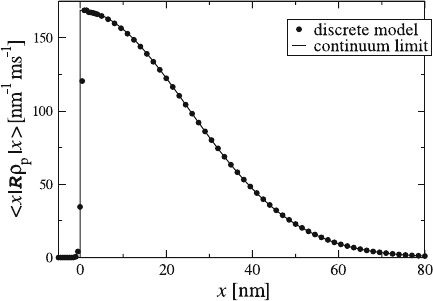
For discrete case, with N = 15 boson modes and χ(x) = Θ(x), the dots in

Fig. 6.14 represent numerical results for



Rρ





for a Gaussian state ρ

|ψψ|. The dots are obtained by a very time-consuming calculation.

In the continuum limit, with the Markov property, and a pure state ρ

=|ψψ|

the reset state is again pure and one obtains

Rρ

=|ψ

reset

ψ

reset

| , (6.157)

with

|ψ

reset

≡A

1/2

χ(

x)|ψ . (6.158)

Fig. 6.14 Dots: N = 15 discrete boson modes, χ(x) = Θ(x); reset state



Rρ





for a Gaussian

state ρ

=|ψ ψ|; solid line: Same with QJA for continuum limit, N →∞, the numerical

evaluation is much faster

170 G.C. Hegerfeldt

This means that after its detection, which is equivalent to the detection of a boson,

the particle state is localized in the region of the detector (given by the sensitivity

function χ (x)). This is a physically very appealing result since a position measure-

ment should localize the particle.

For the continuum limit of the discrete case in Fig. 6.14, the solid curve displays



Rρ





=|x|ψ

reset

|

. The agreement between the discrete version and the QJA

result is excellent. The numerical evaluation of the QJA result, however, is again not

only much faster but almost trivial, by (6.158).

These results and their extensions to many spins have been applied to the study

of arrival and passage times in [27, 28, 41] where more details can be found. In par-

ticular the backreaction of the detection of a boson on the particle has been studied

by the QJA. Somewhat surprisingly it turns out that in spite of the presence of the

spin system mediating between boson and particle this backreaction is not trivial

and of similar nature as in the atom–photon model of Sect. 6.7.2.

6.9 Discussion

In general, a quantum mechanical description of the time development of a sin-

gle system is not possible since quantum mechanics deals with ensembles. But

for a single ﬂuorescing system, like an atom in a trap, which is driven by a light

source and on which photon detections are performed, this is at least partially fea-

sible and it is just accomplished by the quantum jump approach (QJA). Technically

it is achieved by reverting back to an ensemble description. Besides the statisti-

cal properties of the photon detections the QJA also allows one to calculate the

temporal state of the single system depending on the, in principle unpredictable,

stochastic detection times, with a smooth “conditional” time development by a con-

ditional complex Hamiltonian between detections and a reset operation (“jump”)

of the state right thereafter. From this one can determine the statistical proper-

ties of a single radiating system. The temporal succession of continuously chang-

ing states and sudden state reset operations (jumps) of the state at random times

form a quantum trajectory of a given single system. Correspondingly, an ensemble

of many radiating systems determines an ensemble of quantum trajectories. The

related question of whether a single quantum trajectory cannot just be viewed as a

preparation of an ensemble by repetition after each jump or reset will be discussed

below.

In principle one should also realize that there is a distinction between the state-

ments “no photon until time t” and “no photon at time t.” From the theoretical

point of view one therefore has to make sure that there are no photons in between

detections. To ensure this one would, in principle, have to use continuous measure-

ments. In order to avoid this complication and to simplify the approach, the deriva-

tion is proceeded by rapidly repeated, hypothetical (“gedanken”) measurements at

times Δt apart and then invoked temporal coarse graining. Ideally, of course, one

would like to let Δt tend to 0, but with the reduction rule of von Neumann and

uders employed here this is not possible, due to the so-called quantum Zeno effect.

6 The Quantum Jump Approach and Some of Its Applications 171

Therefore, one has to ensure that, within a certain range, the results are independent

of the particular choice of Δt. This can indeed be veriﬁed if the Markov property

holds for the system coupled to the photons (or to another bath). In the derivation

presented in Sect. 6.2 this became particularly transparent because in second-order

perturbation theory the interaction with the bath produced, by the Markov property,

a term proportional to Δt and not to (Δt)

. The latter form of dependence only

sets in for Δt → 0 and gives rise to the quantum Zeno effect. As mentioned in

Sect. 6.2, however, the use of perturbation theory is not essential to the derivation

and that therefore possible errors do not add up for the hypothetical measurements.

Moreover, after the calculation is performed, the probability of ﬁnding no photon

until and at time t turns out to be the same. Physically this can be understood as the

fact that once the photon is away from the atom it is not reabsorbed. Again this can

be shown mathematically to be a consequence of the Markov property, and it would

not hold in a cavity where revivals can occur.

If the Markov property does not hold and if one uses a sequence of gedanken

measurements which are some more or less arbitrary time Δt apart, one will usu-

ally be led to nonphysical results. As another example, in addition to cavities, the

Markov property also does not hold for photonic crystals, due to a photonic band

gap.

When one applies the QJA in simulations it is not necessary to simulate each

of the rapidly repeated individual measurements at times Δt apart, but one can

rather use the conditional Hamiltonian to calculate the waiting time distribution and

generate the detection (or jump) times. Only if this is too complicated, e.g., for a

large number of degrees of freedom coming from many levels or from inclusion of

the atomic motion, one will simulate each time step Δt. The advantage of the QJA

for simulations becomes particularly pronounced if one can work with pure states

because this reduces the dimension to N, i.e., to the number of levels, compared to

for density matrices as in the optical Bloch equations. As has been pointed out

in Sect. 6.6 it is always possible to go over to pure states, even if the reset operation

originally gave a density matrix. The ensemble of quantum trajectories correspond-

ing to an ensemble of radiating systems provides a solution of the optical Bloch

equation for the system, and hence in this respect simulations can be extremely

useful for large N.

The hypothetical, gedanken, measurements employed in the derivation of the

QJA are obviously highly idealized. A realistic photon detector misses many pho-

tons, be it by an efﬁciency less than 1, be it by an aperture less than 4π . The under-

lying assumption is that in such a case the experimental probability distribution is

obtained from the ideal jump (detection) trajectory by assigning, as in [6], probabil-

ities for the recording of the jumps and that one does not need to model the actual

detector in detail.

A variant of the QJA arises in the investigation of the frequency spectrum in a

light period of the Dehmelt system in Fig. 6.1. Here the theoretical problem is that

in order to make sure that one is in a light period one has to detect the photons.

This detection possibly changes the spectrum. In [33] this problem was solved by

measuring the light period through photons emitted in a half space and using it to

172 G.C. Hegerfeldt

trigger a spectrometer in the other half space. This procedure bypasses the time–

energy uncertainty relation.

There is an interesting application of the QJA to an experiment on the quantum

Zeno effect. In the experiment [36] a large number of ions with a V conﬁguration

as in Fig. 6.1 were stored in a Penning trap. The time development was given by

a so-called π pulse of length T

connecting the ground state 1 and the metastable

state 3. Intermittently the ground state population was measured by a very short

pulse of a probe laser coupling level 1 with level 2, where emission of photons

would indicate the ground as measurement outcome and level 3 otherwise. This

was regarded in [36] as a measurement to which the projection postulate could be

applied. With up to 64 probe pulses (“measurements”) during a π pulse agreement

was found, within the error bars, with the quantum Zeno predictions for the level

populations. In an application of the QJA [5], on the other hand, the probe pulse was

directly included into the dynamics and it was shown by means of the QJA that the

probe pulse can indeed be regarded as a measurement which at least approximately

satisﬁes the projection postulate. It was also possible to calculate the errors which

arise when one replaces the probe pulse by an ideal measurement satisfying the

projection postulate.

This is an example of a Heisenberg cut, where part of the measurement apparatus

is included in the dynamics, the actual measurement then being on the photons.

Of course, in the QJA one also employs the projection postulate, but only for the

photons, and the photons are, so to speak, at the very end of the chain. The spin-

boson detector model presented in Sect. 6.8 can be regarded as another example for

a Heisenberg cut. Here the bath of spins can be either viewed as part of the apparatus

or as part of the quantum mechanical system. The spin-boson detector model also

illustrates the fact that the QJA can be applied to a variety of systems which are

coupled to a chain of baths and where the gedanken measurements are performed

on the last member of the chain.

When the resetting in a quantum trajectory is always done to the same state, e.g.,

to the ground state, and if the light source is constant in time, then the trajectory

parts between jumps can be viewed as a preparation of an atomic ensemble by repe-

tition, albeit at random times and of different lengths. There is also a non-Hermitian

conditional time development in this part which is not given by the usual Hermi-

tian Hamiltonian. Such a part of a quantum trajectory corresponds to a complete

system consisting of the driven atom interacting with the quantized radiation ﬁeld

on which rapidly repeated photon measurements are performed with null outcome.

The resetting of the system after the detection of a photon at some random time can

be regarded as a new preparation. In view of the non-Hermitian time development

between resettings this particular ensemble cannot be regarded as a usual ensemble

of atoms plus ﬁeld developing in time since the successive, rapidly repeated, null

measurements between photon detections change the time development. When the

reset operation is not always to the same state, but rather dependent on the condi-

tional state immediately before a photon detection and thus dependent on the prior

history of the trajectory, then the trajectory parts between jumps can also be regarded

Muga G. Time in Quantum Mechanics - Vol. 2

Подождите немного. Документ загружается.