Muga G. Time in Quantum Mechanics

Подождите немного. Документ загружается.

12 Optimal Time Evolution for Hermitian and Non-Hermitian Hamiltonians 347

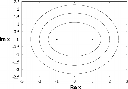
Fig. 12.1 Classical trajectories in the complex-x plane for the harmonic oscillator whose Hamil-

tonian is H = p

+ x

. These trajectories represent the possible paths of a particle whose energy

is E = 1. The trajectories are nested ellipses with foci located at the turning points at x =±1. The

real line segment (degenerate ellipse) connecting the turning points is the usual periodic classical

solution to the harmonic oscillator. All closed paths have the same period 2π

x = a. This trip will take less time because the particle travels faster along the

ellipse in the complex plane.

We have arrived at the surprising conclusion that if the classical particle enters

the parabolic potential V (x) = x

immediately after it begins its voyage up the real

axis, its time of ﬂight will be exactly half a period, or π . Indeed, by traveling in the

complex plane, a particle of energy E = 1 can go from the point x =−a to the

point x = a in time π, no matter how large a is. Evidently, if a particle is allowed to

follow complex classical trajectories, then it is possible to make a drastic reduction

in its time of ﬂight between two given real points.

12.4 Hermitian Quantum Brachistochrone

The quantum brachistochrone problem, as described brieﬂy in Sect. 12.1, is similar

to the classical counterpart except that the optimization takes place in a Hilbert

space. Speciﬁcally, we are given a pair of quantum states, an initial state |ψ

 and

the ﬁnal state |ψ

, and we would like to ﬁnd the one-parameter family of unitary

operators {U

} that achieves the transformation |ψ

→|ψ

=U

|ψ

 in the

smallest possible time t. Since a one-parameter family of unitary operators can be

formed in terms of a Hermitian operator H as U

= exp(−iHt/), the problem

is equivalent to ﬁnding the Hermitian operator H that realizes the transformation

|ψ

→|ψ

 in the shortest possible time.

The Hermitian operator H can be thought of as representing the Hamiltonian, so

the quantum brachistochrone problem is equivalent to ﬁnding the optimal Hamil-

tonian H satisfying exp(−iHt/)|ψ

=|ψ

. However, it is intuitively clear that

if we are allowed to have access to an unbounded energy resource, then the time

348 C.M. Bender and D.C. Brody

required for the relevant transformation, irrespective of whether the Hamiltonian is

optimal or not, can be made arbitrarily small. Hence, for a quantum brachistochrone

problem to possess a nontrivial solution, some form of constraint is needed. The

simplest constraint is to assume that the energy is bounded so that the difference

between the largest and the smallest energy eigenvalues has a ﬁxed value ω:

max

− E

min

= ω. (12.4)

A short calculation shows that if the Hamiltonian H is bounded, then (i) the standard

deviation of the energy is bounded according to

ΔH ≤

max

− E

min

) , (12.5)

and (ii) the state with maximum energy uncertainty is (|E

max

+|E

min

)/

√

2. It

follows that the energy constraint (12.4) is equivalent to a constraint on energy

uncertainty.

The brachistochrone problem of this type has been analyzed recently and a solu-

tion was obtained by means of a variational method [27]. It has also been solved in

terms of a more elementary approach making use of the geometry of quantum state

space [20, 21]. We shall follow closely the latter approach here.

Let us now state the simplest form of the quantum brachistochrone problem:

We have a quantum system represented by an N -dimensional Hilbert space H and

a prescribed pair of states |ψ

 and |ψ

 on H. The problem is (a) to ﬁnd the

Hamiltonian H satisfying the constraint (12.4) such that the unitary transformation

exp(−iHt/)|ψ

=|ψ

 is achieved in the shortest possible time and (b) to ﬁnd

the time required to realize such an operation.

A little geometric intuition allows us to ﬁnd the solution to this problem with

minimum effort. Recall that the time required for transporting a state along a path in

His given by the distance divided by the speed. Hence, all we have to do is ﬁrst iden-

tify the shortest path and measure its length and then allow the state to evolve along

the path with the greatest possible speed without violating the constraint (12.4).

In quantum mechanics the notion of distance is closely linked to the notion of

transition probability [22, 43]. In particular, by looking at the transition probability

between neighboring states we can derive the expression for the metric on the space

of quantum states. This allows us to measure distances between states. The idea can

be sketched as follows: Consider a state |ψin Hand a neighboring state |ψ+|dψ.

The transition probability between these states is

cos





(ψ|+dψ|)|ψψ|(|ψ+|dψ)

ψ|ψ(ψ|+dψ|)(|ψ+|dψ)

, (12.6)

where ds deﬁnes the line element on the space of pure states. By using

cos





≈ 1 −

, (12.7)

12 Optimal Time Evolution for Hermitian and Non-Hermitian Hamiltonians 349

expanding the right side of (12.6), and retaining terms of quadratic order, we ﬁnd

that the line element is

= 4

ψ|ψdψ|dψ−ψ|dψdψ|ψ

ψ|ψ

. (12.8)

This line element is known in geometry to arise from the Fubini–Study metric [47]

and it can be used to measure the distance of the shortest path joining a pair of points

on the space of pure quantum states.

If the Hilbert space is two dimensional, then a generic normalized state vector

|ψ can be expressed in the form

|ψ=

⎛

⎝

cos

sin

θ e

iφ

⎞

⎠

. (12.9)

A short calculation then shows that the Fubini–Study line element (12.8) reduces in

this case to the expression

= dθ

+sin

θ dφ

, (12.10)

which we recognize as the line element on the Bloch sphere S. (The Bloch sphere

is the state space of two-level systems.)

In the case of an N-dimensional Hilbert space H, if we are given a pair of dis-

tinct states |ψ

 and |ψ

, then the linear span of these two states forms a two-

dimensional subspace of H. It should be intuitively clear that the shortest path join-

ing |ψ

and |ψ

should lie on this two-dimensional subspace. Thus, irrespective of

the dimensionality of H the solution to our quantum brachistochrone problem can

be obtained by analyzing the two-dimensional subspace spanned by |ψ

 and |ψ

.

Even when we restrict our attention to this subspace, there still remain inﬁnitely

many unitary orbits that realize the transformation |ψ

→|ψ

=U

|ψ

.How-

ever, since the two-dimensional state space is just the Bloch sphere S endowed with

the spherical metric (12.10), we see that there is a unique great circle arc that joins

|ψ

 and |ψ

 on S. (This assumes, of course, that |ψ

 and |ψ

 are not antipodal

points of the sphere. Otherwise, there are inﬁnitely many such paths.) In this way

we have identiﬁed the shortest path joining |ψ

 and |ψ

. The shortest distance

min

between these two points of S is thus given by

min

= 2 arccos



|ψ

|ψ

|

√

ψ

|ψ

ψ

|ψ



. (12.11)

This result can also be obtained by integrating the line element (12.10) along the

great circle arc on S.

Having obtained the distance of the shortest path we proceed to ﬁnd the max-

imum speed at which the state can evolve unitarily. For the evolution of the state

350 C.M. Bender and D.C. Brody

we must consider the general Schr

odinger equation, but we also need to express the

equation in the correct form. This is the so-called modiﬁed Schr

odinger equation

d|ψ



=−



H|ψ

 . (12.12)

In this equation the mean-adjusted Hamiltonian

H is given by

H = H −H , (12.13)

where

H=

ψ|H|ψ

ψ|ψ

. (12.14)

Note that 

H=0 and that according to (12.12) the tangent vector

|ψ

 is every-

where orthogonal to the direction of the state [46]. Since the energy expectation H

depends on the state |ψ, the modiﬁed Schr

odinger equation appears to be nonlinear.

However, this is not the case. The point is that the expectation value of the Hamil-

tonian is a constant of the motion under the Schr

odinger dynamics. Thus, given the

initial state |ψ

, we calculate H in this state and subtract this number from the

Hamiltonian. Since the Hamiltonian in quantum mechanics is deﬁned only up to

an additive constant, this modiﬁcation does not alter the physics in any way. It is

worthwhile noting that the modiﬁed Schr

odinger equation (12.12) is canonical and

reduces to the standard eigenvalue problem when the state |ψ

 is time independent

without one having to evoke the correspondence principle [22].

If the initial state vector |ψ

 is normalized, then the evolution (12.12) preserves

the norm. It follows that ψ|dψ=0. Since the speed v of quantum evolution is

given by v = ds/dt, we ﬁnd from (12.8) and (12.12) that



ψ

|(H −H)

|ψ

=



ψ

|(H −H)

|ψ

 . (12.15)

This shows that the speed of quantum evolution is given by the energy uncer-

tainty. The expression (12.15) for the speed of quantum evolution is known as

the Anandan–Aharonov relation [1]. Since we know from (12.5) that under the

constraint (12.4) the energy uncertainty ΔH is bounded by

ω, we ﬁnd that the

maximum speed of quantum evolution is given by

max



. (12.16)

By using the results in (12.11) and (12.16) we deduce that the minimum time

required for realizing the unitary transportation |ψ

→|ψ

=U

|ψ

 is given

by the ratio s

min

max

. In particular, if |ψ

 and |ψ

 are orthogonal, then they

correspond to antipodal points on the Bloch sphere S, and we have s

min

= π .In

12 Optimal Time Evolution for Hermitian and Non-Hermitian Hamiltonians 351

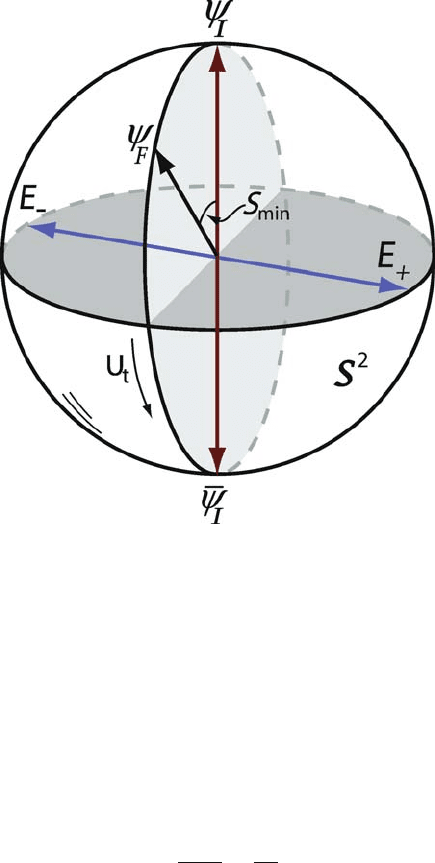
Fig. 12.2 (Color online) Optimal Hamiltonian for quantum state transportation. The two-

dimensional complex Hilbert space spanned by the initial state |ψ

 and the ﬁnal state |ψ

 can be

visualized in real terms as a Bloch sphere S. The two states |ψ

 and |ψ

 can then be identiﬁed

as a pair of points on S. Assuming that these two points are not antipodal, there exists a unique

great circle arc joining these two points, which determines the shortest path joining the two states.

The optimal way of unitarily transporting |ψ

 into |ψ

 is therefore to rotate the sphere along the

axis orthogonal to the great circle. The axis of rotation then speciﬁes two quantum states: |E

−

and

. These states are the eigenstates of the optimal Hamiltonian H

this case, the minimum time required to orthogonalize the state (that is, for the state

to evolve into a new state that is orthogonal to the original state) is known as the

passage time τ

[19, 59]. The passage time is explicitly

π

2ΔH

π

. (12.17)

The passage time (12.17) provides the bound in Hermitian quantum mechanics for

transporting a state into an orthogonal state and is sometimes referred to as the

Fleming bound [33].

The ratio s

min

max

gives the solution to part (b) of our quantum brachistochrone

problem. To solve part (a), that is, to ﬁnd the optimal Hamiltonian, we argue as

follows: Since the problem is conﬁned to a two-dimensional subspace of H,the

solution can be obtained by elementary trigonometry on the Bloch sphere S.The

352 C.M. Bender and D.C. Brody

key idea is to recall that the shortest path joining |ψ

 and |ψ

 is a great circle

arc on S. Without loss of generality, we can assume that |ψ

 and |ψ

 lie on the

equator of S with respect to a suitable choice of axis. Then, the unitary motion

along the shortest path can be generated by the rotation of S along this axis. Since

the eigenstates of the Hamiltonian H that generates such a rotation correspond to

the antipodal points along this axis, the pair of states |ψ

 and |ψ

 can both be

expressed as equal superpositions of the eigenstates of H with the relative phase

shifted by s

min

. Writing |E

 and |E

−

 for the normalized eigenstates of H and

using α = s

min

/2, we can express the initial and ﬁnal states in the form

√



−

+e

−iα





=|ψ

 and

√



−

+e

iα





=|ψ

 . (12.18)

Solving these equations for |E

 and |E

−

, we obtain

−

=

√

2sinα



−iα

|ψ

−e

iα

|ψ





(12.19)

and

=−

√

2sinα



|ψ

−|ψ





. (12.20)

These are the eigenstates of the optimal Hamiltonian H that generate the unitary

motion |ψ

→|ψ

=U

|ψ

 along the shortest path. The eigenvalues of the

optimal H can be arbitrary as long as condition (12.4) is satisﬁed. Without loss of

generality, we may assume H to be trace free, and we obtain the solution to part (a)

of the quantum brachistochrone problem:

H =

ω|E

E

|−

ω|E

−

E

−

| . (12.21)

This is the “minimal” solution to the problem in the sense that H acts only on the

two-dimensional subspace of H while leaving the rest of H unperturbed.

As a special example, consider the problem of a spin ﬂip, that is, turning a spin-up

state into a spin-down state unitarily. In this case the initial and ﬁnal states can be

written as

|ψ

=





and |ψ

=





(12.22)

in the spin-z basis. Substituting these into (12.19) and (12.20), we ﬁnd that the

eigenstates of the optimal Hamiltonian are

−

=

√





and |E

=

√



−1



(12.23)

because in this case we have α = π/2. Substituting this result into (12.21) yields

12 Optimal Time Evolution for Hermitian and Non-Hermitian Hamiltonians 353

H =



0 −ω

−ω 0



(12.24)

for the optimal Hamiltonian. By using the relation

iφσ·n

= cos φ1 + isinφσ ·n , (12.25)

where n is a unit vector and





, σ



0 −i

i 0



, σ



0 −1



(12.26)

are Pauli matrices, we obtain the following expression for the optimal unitary oper-

ator:

⎛

⎝

cos



ωt

2



−isin



ωt

2



−isin



ωt

2



cos



ωt

2



⎞

⎠

. (12.27)

It follows at once that the optimal unitary orbit |ψ

=U

|ψ

 is given by

|ψ

=

cos



ωt

2



−isin



ωt

2



. (12.28)

We ﬁnd that the ﬁrst time at which |ψ

 reaches |ψ

 is given by the condition

ωt/2 = π/2, that is, when t = τ

, where τ

is the passage time given in (12.17).

We have seen how the simplest form of a quantum brachistochrone problem

can be solved in Hermitian quantum mechanics by considering a two-dimensional

Hilbert subspace combined with elementary geometric constructions on it. In a more

general situation the unitary motion may be constrained further so that the opti-

mal Hamiltonian (12.21) may not be implementable. For example, the constraint

may enforce the path of the unitary evolution to lie in a three- rather than two-

dimensional subspace. To determine what happens let us work out the passage time

for this example.

Since in this case the minimal solution H to the brachistochrone problem is a

three-dimensional matrix, we can express the initial state |ψ

 in terms of the three

eigenstates of H according to

|ψ

=cos α|E

+sin α cos βe

iφ

+sin α sin βe

iϕ

 , (12.29)

where α, β are angular coordinates, φ, ϕ are phase variables, and we assume that

< E

. If a unitary operator U

transforms this state into an orthogonal

state, then the condition

cos

α +sin

α cos

βe

−iω

T/

+sin

α sin

βe

−iω

T/

= 0 (12.30)

354 C.M. Bender and D.C. Brody

must be satisﬁed, where ω

= E

− E

and ω

= E

− E

. To render the anal-

ysis more tractable, we simplify this constraint by assuming that α = β = π/4.

Then (12.30) implies that a necessary condition for the state |ψ

 to evolve into an

orthogonal state is given by the relation

2m − 1

2n − 1

, (12.31)

where m, n are natural numbers such that m = n.

Thus, the solution to the brachistochrone problem must be such that the eigen-

values of H satisfy condition (12.31) as well as the constraint E

max

− E

min

≤ ω.

Assuming that these constraints are indeed satisﬁed, the initial state evolves into

an orthogonal state |ψ

. The ﬁrst time that |ψ

 evolves into a state orthogonal to

|ψ

, in particular, is given by

T =

π

3π

. (12.32)

However, since in this case U

|ψ

 does not describe a geodesic path, T will be

larger than Fleming’s passage time τ

given in (12.17). Indeed, without loss of gen-

erality we may set E

= 0. Then, it is straightforward to verify that T =

√

6τ

.This

follows from the fact that under the constraint ω

= 3ω

that comes from (12.32),

the squared energy dispersion in the state (12.29) with α = β = π/4 is given by

ΔH

12.5 Non-Hermitian Quantum Brachistochrone

We have seen how the solution to the simple brachistochrone problem can be

obtained in the Hermitian quantum theory. What happens if we extend the quantum

theory into the complex domain by looking at a PT-symmetric theory? We saw ear-

lier that in classical mechanics if we were to allow for a complex path interpolating

a pair of real points of the coordinate space, then it is possible (at least mathemati-

cally) to transport a particle across a large distance in virtually no time. It turns out

that an analogous situation emerges in the PT-symmetric theory. Here we present

a simple algebraic calculation of the optimal evolution time from an initial state to

a ﬁnal state by using a simple 2 × 2 Hamiltonian. As we have remarked above,

the 2 × 2 model sufﬁces to cover general cases because in the case of our simple

brachistochrone problem the solution is found on the two-dimensional subspace of

the Hilbert space spanned by the initial state |ψ

 and the ﬁnal state |ψ

.Inthe

case of a PT-symmetric Hamiltonian the variational approach gives a more direct

way to handle the brachistochrone problem. Thus, we shall ﬁrst brieﬂy revisit the

Hermitian case but expressed in the variational formalism and then we will compare

the result to its PT-symmetric counterpart.

12 Optimal Time Evolution for Hermitian and Non-Hermitian Hamiltonians 355

12.5.1 Hermitian 2 × 2 Matrices

We choose a basis so that the initial and ﬁnal state vectors take the form

|ψ

=





and |ψ

=





, (12.33)

where the condition that |ψ

 be normalized is |a|

+|b|

= 1. The most general

2 × 2 Hermitian Hamiltonian is

H =



sre

−iθ

r e

iθ



(r, s, u,θreal) . (12.34)

For this Hamiltonian the eigenvalue constraint (12.4) takes the form

= (s − u)

+4r

. (12.35)

To ﬁnd the optimal Hamiltonian satisfying this constraint, we rewrite H as a

linear combination of Pauli matrices:

H =

(s +u)1 +

ωσ·n , (12.36)

where

n =

(2r cos θ,2r sin θ,s − u) (12.37)

is a unit vector. Then by the use of identity (12.25) the evolution equation |ψ

=

−iHτ/

|ψ

 can be expressed in the form





= e

−

i(s+u)t/

⎛

⎝

cos

ωt

2

−i

s−u

sin

ωt

2

−i

iθ

sin

ωt

2

⎞

⎠

. (12.38)

The second component of this equation gives |b|=

sin

ωt

2

, which allows us to

ﬁnd the required time of evolution:

t =

2

arcsin

ω|b|

. (12.39)

We must now minimize the time t over all r > 0 while maintaining the energy

constraint in (12.35). This constraint tells us that the maximum value of r is

ω.At

this value we have s = u. Because H can be made trace free, we can set s = u = 0.

The variable θ in (12.36) does not affect the eigenvalues, so we may set θ = π. Then

we recover the optimal Hamiltonian obtained in (12.24). As regards the minimum

evolution time τ we have

356 C.M. Bender and D.C. Brody

τ =

2arcsin |b|

. (12.40)

In the special case for which a = 0 and b = 1 so that |ψ

 and |ψ

 are orthogonal,

we recover the passage time τ = τ

= π/ω, the smallest time required for a spin

ﬂip .

Although the form of the result in (12.40) resembles the statement of the uncer-

tainty principle, it is merely the statement indicated above that rate ×time=distance;

the maximum speed of evolution is given by ΔH, and the distance between |ψ



and |ψ

, assuming they are normalized, is given by 2 arccos(|ψ

|ψ

|). Since

|ψ

|ψ

| = |a| and |a|=

1 −|b|

, we obtain (12.40) from the relation

arccos

1 −|b|

= arcsin|b| . (12.41)

12.5.2 Non-Hermitian 2 × 2 Matrices

We now show by direct calculation that for a PT-symmetric Hamiltonian, τ can be

arbitrarily small. This is because a PT-symmetric Hamiltonian whose eigenvalues

are all real is equivalent to a Hermitian Hamiltonian via

H = e

−Q/2

Q/2

, where

Q is Dirac Hermitian. The states in a PT-symmetric theory are mapped by e

−Q/2

to the corresponding states in the Dirac Hermitian theory. But, the overlap distance

between two states does not remain constant under a similarity transformation. We

can exploit this property of the similarity transformation to overcome the Hermitian

lower limit on the time τ . (The detailed calculation is explained in [14].)

We consider the general class of PT-symmetric 2 × 2 Hamiltonians having the

form

H =



r e

iθ

sre

−iθ



(r, s,θreal) . (12.42)

The time-reversal operator T performs complex conjugation and the parity operator

in this case is given by

P =





. (12.43)

The two eigenvalues

= r cos θ ±

−r

sin

θ (12.44)

are real if s

> r

sin

θ. This inequality deﬁnes the region of unbroken PT sym-

metry. The unnormalized eigenstates of H are

Muga G. Time in Quantum Mechanics - Vol. 2

Подождите немного. Документ загружается.