Munson B.R. Fundamentals of Fluid Mechanics
Подождите немного. Документ загружается.

1for shearing stresses2
(6.125d)
(6.125e)
(6.125f)
where p is the pressure, the negative of the average of the three normal stresses; that is,
For viscous fluids in motion the normal stresses are not necessarily the
same in different directions, thus, the need to define the pressure as the average of the three normal
stresses. For fluids at rest, or frictionless fluids, the normal stresses are equal in all directions. 1We
have made use of this fact in the chapter on fluid statics and in developing the equations for inviscid
flow.2Detailed discussions of the development of these stress–velocity gradient relationships can
be found in Refs. 3, 7, and 8. An important point to note is that whereas for elastic solids the
stresses are linearly related to the deformation 1or strain2, for Newtonian fluids the stresses are
linearly related to the rate of deformation 1or rate of strain2.
In cylindrical polar coordinates the stresses for incompressible Newtonian fluids are expressed
as 1for normal stresses2
(6.126a)
(6.126b)
(6.126c)
1for shearing stresses2
(6.126d)
(6.126e)
(6.126f)
The double subscript has a meaning similar to that of stresses expressed in Cartesian coordinates—
that is, the first subscript indicates the plane on which the stress acts, and the second subscript the
direction. Thus, for example, refers to a stress acting on a plane perpendicular to the radial direction
and in the radial direction 1thus a normal stress2. Similarly, refers to a stress acting on a plane
perpendicular to the radial direction but in the tangential 1 direction2and is therefore a shearing stress.
6.8.2 The Navier–Stokes Equations
The stresses as defined in the preceding section can be substituted into the differential equations
of motion 1Eqs. 6.502and simplified by using the continuity equation 1Eq. 6.312to obtain:
1x direction2
(6.127a)
1y direction2
(6.127b) r a
0v
0t
⫹ u
0v
0x
⫹ v
0v
0y
⫹ w
0v
0z
b⫽⫺
0p
0y
⫹ rg
y
⫹ m a
0
2
v
0x
2
⫹
0
2
v
0y
2
⫹
0
2
v
0z
2
b
r a
0u
0t
⫹ u
0u
0x
⫹ v
0u
0y
⫹ w
0u
0z
b⫽⫺
0p
0x
⫹ rg
x
⫹ m a
0
2
u
0x
2
⫹
0
2
u
0y
2
⫹
0
2
u
0z
2
b
u
t
ru
s
rr
t
zr
⫽ t
rz
⫽ m a
0v
r
0z
⫹
0v
z
0r
b
t
uz
⫽ t
zu
⫽ m a
0v
u
0z
⫹
1
r
0v
z
0u
b
t
ru
⫽ t
ur
⫽ m cr
0
0r
a
v
u
r
b⫹
1
r
0v
r
0u
d
s
zz
⫽⫺p ⫹ 2m
0v
z
0z
s
uu
⫽⫺p ⫹ 2m a
1
r
0v
u
0u
⫹
v
r
r
b
s
rr
⫽⫺p ⫹ 2m
0v
r
0r
⫺p ⫽ 1
1
3
21s
xx
⫹ s
yy
⫹ s
zz
2.
t
zx
⫽ t
xz
⫽ m a
0w
0x
⫹
0u
0z
b
t
yz
⫽ t
zy
⫽ m a
0v
0z
⫹
0w
0y
b
t
xy
⫽ t
yx
⫽ m
a
0u
0y
⫹
0v
0x
b
6.8 Viscous Flow 307
For Newtonian
fluids, stresses are
linearly related to
the rate of strain.
y
x
z
w
v
u
JWCL068_ch06_263-331.qxd 9/23/08 12:19 PM Page 307
1z direction2
(6.127c)
where and w are the x, y, and z components of velocity as shown in the figure in the margin
of the previous page. We have rearranged the equations so the acceleration terms are on the left
side and the force terms are on the right. These equations are commonly called the Navier–Stokes
equations, named in honor of the French mathematician L. M. H. Navier 11785–18362and the
English mechanician Sir G. G. Stokes 11819–19032, who were responsible for their formulation.
These three equations of motion, when combined with the conservation of mass equation 1Eq. 6.312,
provide a complete mathematical description of the flow of incompressible Newtonian fluids. We
have four equations and four unknowns and and therefore the problem is “well-posed”
in mathematical terms. Unfortunately, because of the general complexity of the Navier–Stokes
equations 1they are nonlinear, second-order, partial differential equations2, they are not amenable
to exact mathematical solutions except in a few instances. However, in those few instances in which
solutions have been obtained and compared with experimental results, the results have been in close
agreement. Thus, the Navier–Stokes equations are considered to be the governing differential
equations of motion for incompressible Newtonian fluids.
In terms of cylindrical polar coordinates 1see the figure in the margin2, the Navier–Stokes
equations can be written as
1r direction2
(6.128a)
1 direction2
(6.128b)
1z direction2
(6.128c)
To provide a brief introduction to the use of the Navier–Stokes equations, a few of the
simplest exact solutions are developed in the next section. Although these solutions will prove to
be relatively simple, this is not the case in general. In fact, only a few other exact solutions have
been obtained.
⫽⫺
0p
0z
⫹ rg
z
⫹ m c
1
r
0
0r
ar
0v
z
0r
b⫹
1
r
2
0
2
v
z
0u
2
⫹
0
2
v
z
0z
2
d
r a
0v
z
0t
⫹ v
r
0v
z
0r
⫹
v
u
r
0v
z
0u
⫹ v
z
0v
z
0z
b
⫽⫺
1
r
0p
0u
⫹ rg
u
⫹ m c
1
r
0
0r
ar
0v
u
0r
b⫺
v
u
r
2
⫹
1
r
2
0
2
v
u
0u
2
⫹
2
r
2
0v
r
0u
⫹
0
2
v
u
0z
2
d
r a
0v
u
0t
⫹ v
r
0v
u
0r
⫹
v
u
r
0v
u
0u
⫹
v
r
v
u
r
⫹ v
z
0v
u
0z
b
u
⫽⫺
0p
0r
⫹ rg
r
⫹ m
c
1
r
0
0r
ar
0v
r
0r
b⫺
v
r
r
2
⫹
1
r
2
0
2
v
r
0u
2
⫺
2
r
2
0v
u
0u
⫹
0
2
v
r
0z
2
d
r a
0v
r
0t
⫹ v
r
0v
r
0r
⫹
v
u
r
0v
r
0u
⫺
v
2
u
r
⫹ v
z
0v
r
0z
b
p2,1u, v, w,
u, v,
r a
0w
0t
⫹ u
0w
0x
⫹ v
0w
0y
⫹ w
0w
0z
b⫽⫺
0p
0z
⫹ rg
z
⫹ m a
0
2
w
0x
2
⫹
0
2
w
0y
2
⫹
0
2
w
0z
2
b
308 Chapter 6 ■ Differential Analysis of Fluid Flow
The Navier–Stokes
equations are the
basic differential
equations describ-
ing the flow of
Newtonian fluids.
A principal difficulty in solving the Navier–Stokes equations is because of their nonlinearity arising
from the convective acceleration terms There are no general analytical
schemes for solving nonlinear partial differential equations 1e.g., superposition of solutions cannot
be used2, and each problem must be considered individually. For most practical flow problems, fluid
particles do have accelerated motion as they move from one location to another in the flow field.
Thus, the convective acceleration terms are usually important. However, there are a few special cases
for which the convective acceleration vanishes because of the nature of the geometry of the flow
1i.e., u 0u
Ⲑ
0x, w 0v
Ⲑ
0z, etc.2.
6.9 Some Simple Solutions for Laminar, Viscous, Incompressible Fluids
θ
y
x
z
v
v
z
v
r
θ
r
JWCL068_ch06_263-331.qxd 9/23/08 12:19 PM Page 308
system. In these cases exact solutions are often possible. The Navier–Stokes equations apply to both
laminar and turbulent flow, but for turbulent flow each velocity component fluctuates randomly with
respect to time and this added complication makes an analytical solution intractable. Thus, the exact
solutions referred to are for laminar flows in which the velocity is either independent of time 1steady
flow2or dependent on time 1unsteady flow2in a well-defined manner.
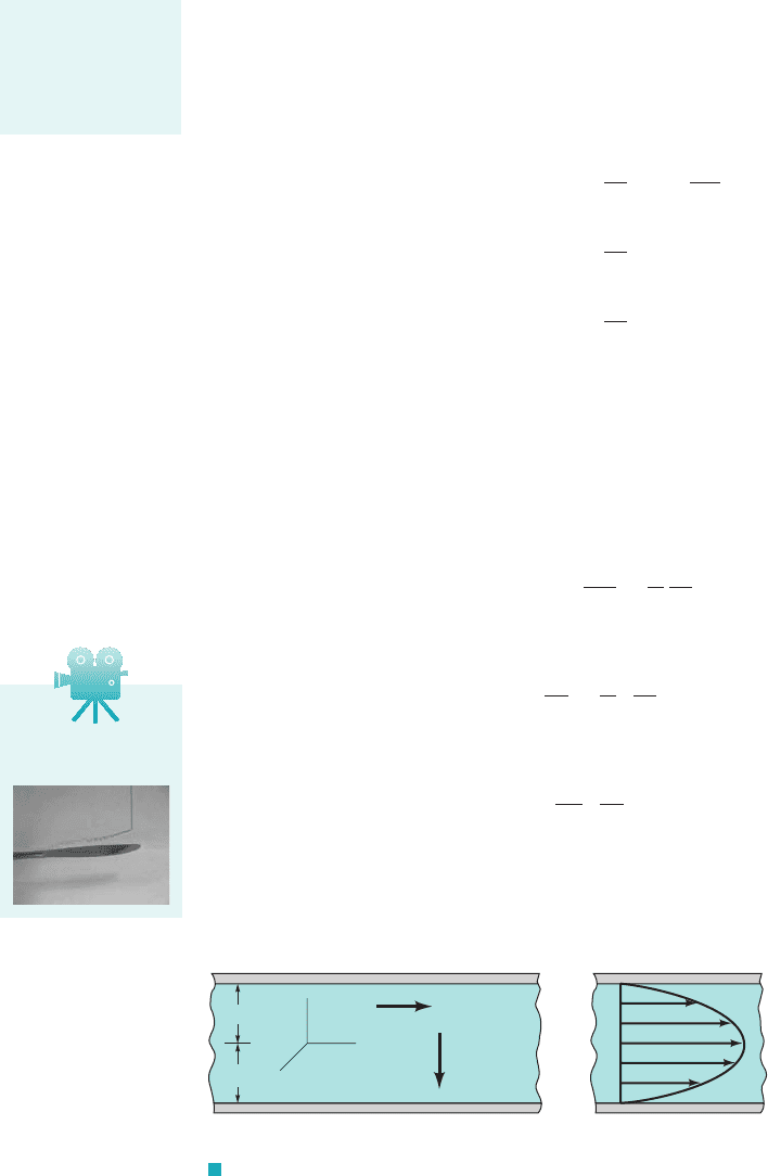
6.9.1 Steady, Laminar Flow between Fixed Parallel Plates
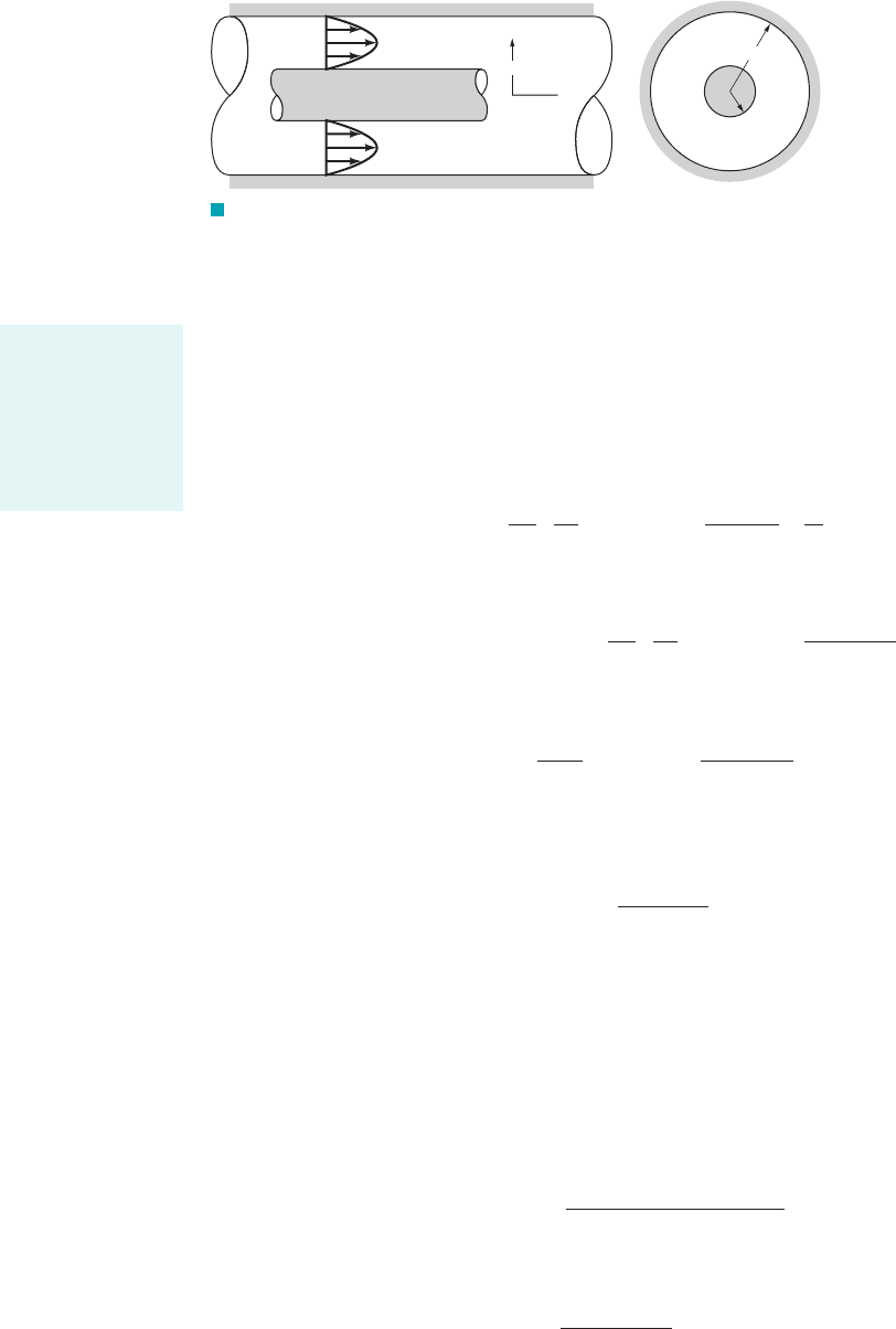
We first consider flow between the two horizontal, infinite parallel plates of Fig. 6.31a. For this
geometry the fluid particles move in the x direction parallel to the plates, and there is no velocity
in the y or z direction—that is, In this case it follows from the continuity equation
1Eq. 6.312that Furthermore, there would be no variation of u in the z direction for
infinite plates, and for steady flow so that If these conditions are used in the
Navier–Stokes equations 1Eqs. 6.1272, they reduce to
(6.129)
(6.130)
(6.131)
where we have set and That is, the y axis points up. We see that for this
particular problem the Navier–Stokes equations reduce to some rather simple equations.
Equations 6.130 and 6.131 can be integrated to yield
(6.132)
which shows that the pressure varies hydrostatically in the y direction. Equation 6.129, rewritten
as
can be integrated to give
and integrated again to yield
(6.133)
Note that for this simple flow the pressure gradient, is treated as constant as far as the
integration is concerned, since 1as shown in Eq. 6.1322it is not a function of y. The two constants
must be determined from the boundary conditions. For example, if the two plates arec
1
and c
2
0p
Ⲑ
0x,
u ⫽
1
2m
a
0p
0x
b y
2
⫹ c
1
y ⫹ c
2
du
dy
⫽
1
m
a
0p
0x
b y ⫹ c
1
d
2
u
dy
2
⫽
1
m
0p
0x
p ⫽⫺rgy ⫹ f
1
1x2
g
z
⫽ 0.g
x
⫽ 0, g
y
⫽⫺g,
0 ⫽⫺
0p
0z
0 ⫽⫺
0p
0y
⫺ rg
0 ⫽⫺
0p
0x
⫹ m a
0
2
u
0y
2
b
u ⫽ u1y2.0u
Ⲑ
0t ⫽ 0
0u
Ⲑ
0x ⫽ 0.
v ⫽ 0 and w ⫽ 0.
6.9 Some Simple Solutions for Laminar, Viscous, Incompressible Fluids 309
An exact solution
can be obtained for
steady laminar flow
between fixed paral-
lel plates.
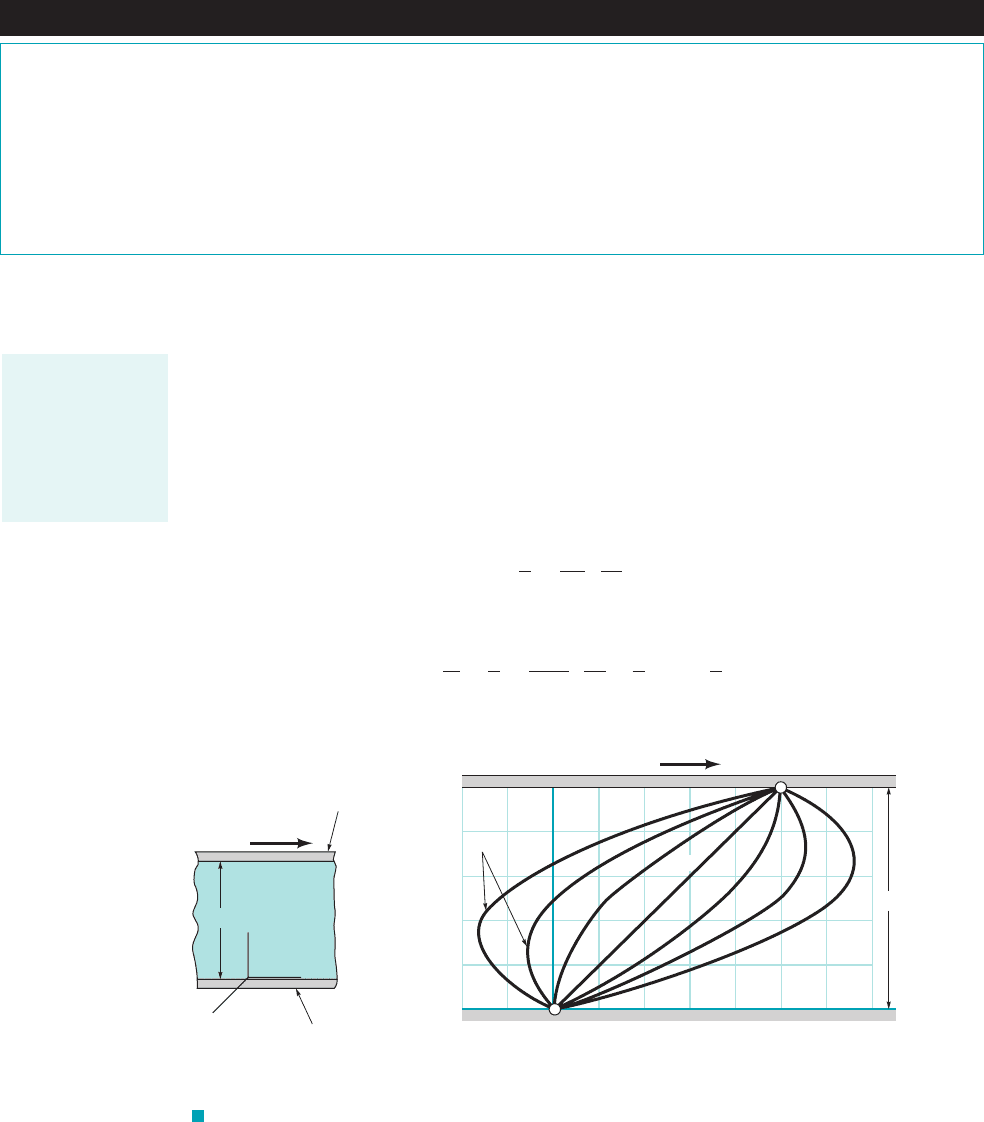
u
g
h
h
z
x
y
u
u
max
(a)(b)
F I G U R E 6.31 The viscous flow between parallel plates:
(a) coordinate system and notation used in analysis; (b) parabolic velocity
distribution for flow between parallel fixed plates.
V6.11 No-slip
boundary condition
JWCL068_ch06_263-331.qxd 9/23/08 12:19 PM Page 309
fixed, then for 1because of the no-slip condition for viscous fluids2. To satisfy this
condition and
Thus, the velocity distribution becomes
(6.134)
Equation 6.134 shows that the velocity profile between the two fixed plates is parabolic as illustrated
in Fig. 6.31b.
The volume rate of flow, q, passing between the plates 1for a unit width in the z direction2is
obtained from the relationship
or
(6.135)
The pressure gradient is negative, since the pressure decreases in the direction of flow. If
we let represent the pressure drop between two points a distance apart, then
and Eq. 6.135 can be expressed as
(6.136)
The flow is proportional to the pressure gradient, inversely proportional to the viscosity, and strongly
dependent on the gap width. In terms of the mean velocity, V, where Eq. 6.136
becomes
(6.137)
Equations 6.136 and 6.137 provide convenient relationships for relating the pressure drop along a
parallel-plate channel and the rate of flow or mean velocity. The maximum velocity, occurs
midway between the two plates, as shown in Fig. 6.31b, so that from Eq. 6.134
or
(6.138)
The details of the steady laminar flow between infinite parallel plates are completely predicted
by this solution to the Navier–Stokes equations. For example, if the pressure gradient, viscosity, and
plate spacing are specified, then from Eq. 6.134 the velocity profile can be determined, and from
Eqs. 6.136 and 6.137 the corresponding flowrate and mean velocity determined. In addition, from
Eq. 6.132 it follows that
where is a reference pressure at and the pressure variation throughout the fluid can
be obtained from
(6.139)p rgy a
0p
0x
b x p
0
x y 0,p
0
f
1
1x2 a
0p
0x
b x p
0
u
max
3
2
V
u
max
h
2
2m
a
0p
0x
b
1y 02
u
max
,
V
h
2
¢p
3m/
V q
2h,1⬃h
3
2
q
2h
3
¢p
3m/
¢p
/
0p
0x
/¢p
0p
0x
q
2h
3
3m
a
0p
0x
b
q
冮
h
h
u dy
冮
h
h
1
2m
a
0p
0x
b 1y
2
h
2
2
dy
u
1
2m
a
0p
0x
b 1y
2
h
2
2
c
2
1
2m
a
0p
0x
b h
2
c
1
0
y hu 0
310 Chapter 6 ■ Differential Analysis of Fluid Flow
V6.12 Liquid–
liquid no-slip
The Navier–Stokes
equations provide
detailed flow char-
acteristics for lami-
nar flow between
fixed parallel plates.
JWCL068_ch06_263-331.qxd 9/23/08 12:19 PM Page 310
For a given fluid and reference pressure, the pressure at any point can be predicted. This relatively
simple example of an exact solution illustrates the detailed information about the flow field which
can be obtained. The flow will be laminar if the Reynolds number, remains below
about 1400. For flow with larger Reynolds numbers the flow becomes turbulent and the preceding
analysis is not valid since the flow field is complex, three-dimensional, and unsteady.
Re ⫽ rV12h2
Ⲑ
m,
p
0
,
6.9 Some Simple Solutions for Laminar, Viscous, Incompressible Fluids 311
Fluids in the News
10 tons on 8 psi Place a golf ball on the end of a garden hose
and then slowly turn the water on a small amount until the ball
just barely lifts off the end of the hose, leaving a small gap be-
tween the ball and the hose. The ball is free to rotate. This is the
idea behind the new “floating ball water fountains” developed
in Finland. Massive, 10-ton, 6-ft-diameter stone spheres are
supported by the pressure force of the water on the curved sur-
face within a pedestal and rotate so easily that even a small
child can change their direction of rotation. The key to the
fountain design is the ability to grind and polish stone to an ac-
curacy of a few thousandths of an inch. This allows the gap be-
tween the ball and its pedestal to be very small (on the order of
5/1000 in.) and the water flowrate correspondingly small (on
the order of 5 gallons per minute). Due to the small gap, the
flow in the gap is essentially that of flow between parallel
plates. Although the sphere is very heavy, the pressure under
the sphere within the pedestal needs to be only about 8 psi. (See
Problem 6.88.)
6.9.2 Couette Flow
Another simple parallel-plate flow can be developed by fixing one plate and letting the other plate
move with a constant velocity, U, as is illustrated in Fig. 6.32a. The Navier–Stokes equations
reduce to the same form as those in the preceding section, and the solution for the pressure and
velocity distribution are still given by Eqs. 6.132 and 6.133, respectively. However, for the moving
plate problem the boundary conditions for the velocity are different. For this case we locate the
origin of the coordinate system at the bottom plate and designate the distance between the two
plates as b 1see Fig. 6.32a2. The two constants and in Eq. 6.133 can be determined from the
boundary conditions, at and at It follows that
(6.140)
or, in dimensionless form,
(6.141)
u
U
⫽
y
b
⫺
b
2
2mU
a
0p
0x
b a
y
b
b a1 ⫺
y
b
b
u ⫽ U
y
b
⫹
1
2m
a
0p
0x
b 1y
2
⫺ by2
y ⫽ b.u ⫽ Uy ⫽ 0u ⫽ 0
c
2
c
1
U
U
1.0
0.8
0.6
0.4
0.2
-0.4 -0.2 0 0.2 0.4 0.6 0.8 1.0 1.2 1.4
b
3210–1–2
P = –3
Back-
flow
y
_
b
u
__
U
(b)(a)
Fixed
plate
z
x
y
b
Moving
plate
0
F I G U R E 6.32 The viscous flow between parallel plates with bottom plate fixed and
upper plate moving (Couette flow): (a) coordinate system and notation used in analysis; (b) velocity
distribution as a function of parameter, P, where ( ) (From Ref. 8, used by
permission.)
p兾x.b
2
兾2MUP
For a given flow
geometry, the char-
acter and details of
the flow are
strongly dependent
on the boundary
conditions.
JWCL068_ch06_263-331.qxd 9/23/08 12:19 PM Page 311
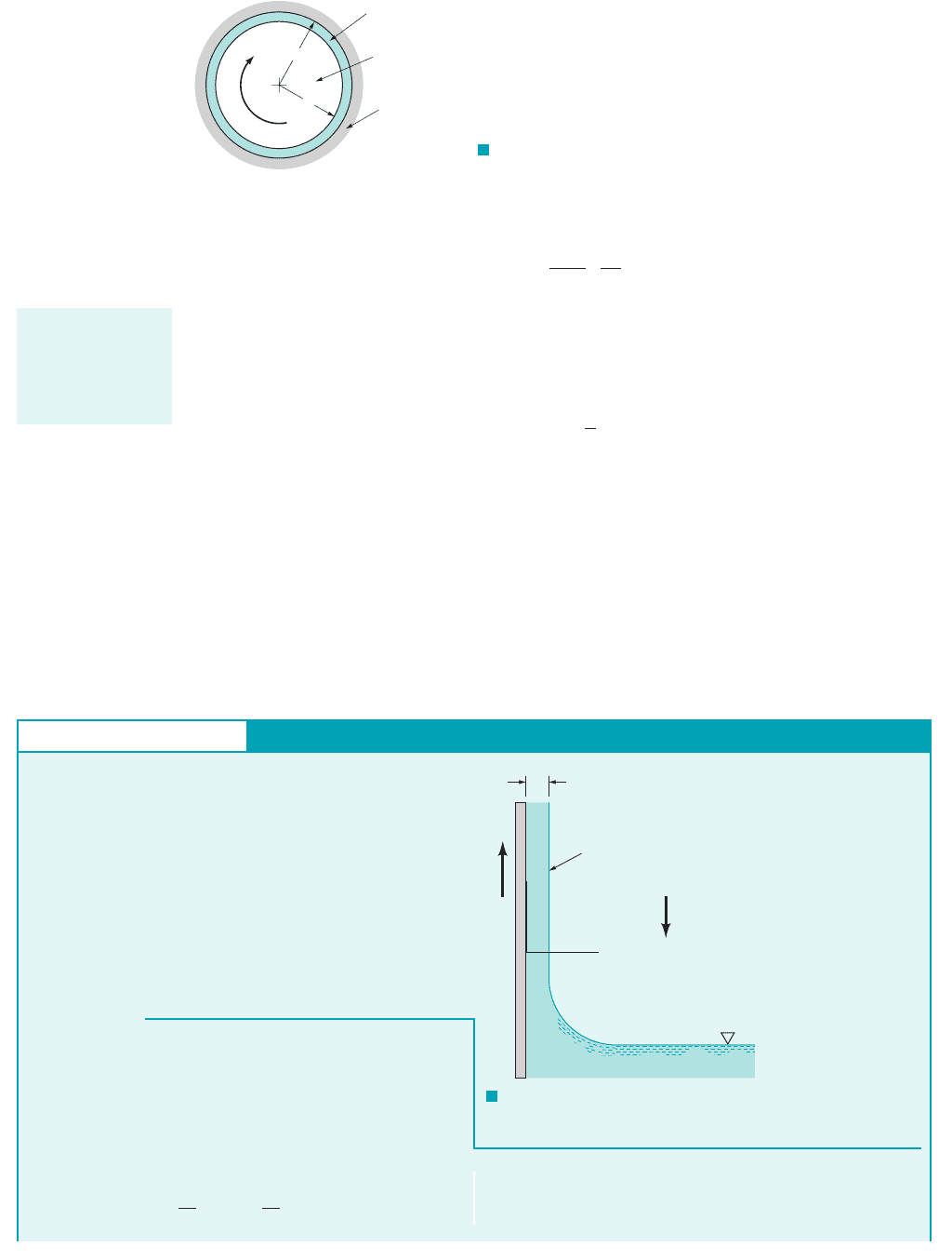
The actual velocity profile will depend on the dimensionless parameter
Several profiles are shown in Fig. 6.32b. This type of flow is called Couette flow.
The simplest type of Couette flow is one for which the pressure gradient is zero; that is, the
fluid motion is caused by the fluid being dragged along by the moving boundary. In this case, with
Eq. 6.140 simply reduces to
(6.142)
which indicates that the velocity varies linearly between the two plates as shown in Fig. 6.31b for
This situation would be approximated by the flow between closely spaced concentric cylinders
in which one cylinder is fixed and the other cylinder rotates with a constant angular velocity, As
illustrated in Fig. 6.33, the flow in an unloaded journal bearing might be approximated by this simple
Couette flow if the gap width is very small In this case and
the shearing stress resisting the rotation of the shaft can be simply calculated as
When the bearing is loaded 1i.e., a force applied normal to the axis of rotation2, the shaft will no longer
remain concentric with the housing and the flow cannot be treated as flow between parallel boundaries.
Such problems are dealt with in lubrication theory 1see, for example, Ref. 92.
t mr
i
v
1r
o
r
i
2.
U r
i
v, b r
o
r
i
,1i.e., r
o
r
i
r
i
2.
v.
P 0.
u U
y
b
0p
0x 0,
P
b
2
2mU
a
0p
0x
b
312 Chapter 6 ■ Differential Analysis of Fluid Flow
Flow between par-
allel plates with one
plate fixed and the
other moving is
called Couette flow.
ω
r
i
r
o
Lubricating
oil
Rotating shaft
Housing
F I G U R E 6.33 Flow in the narrow gap of a
journal bearing.
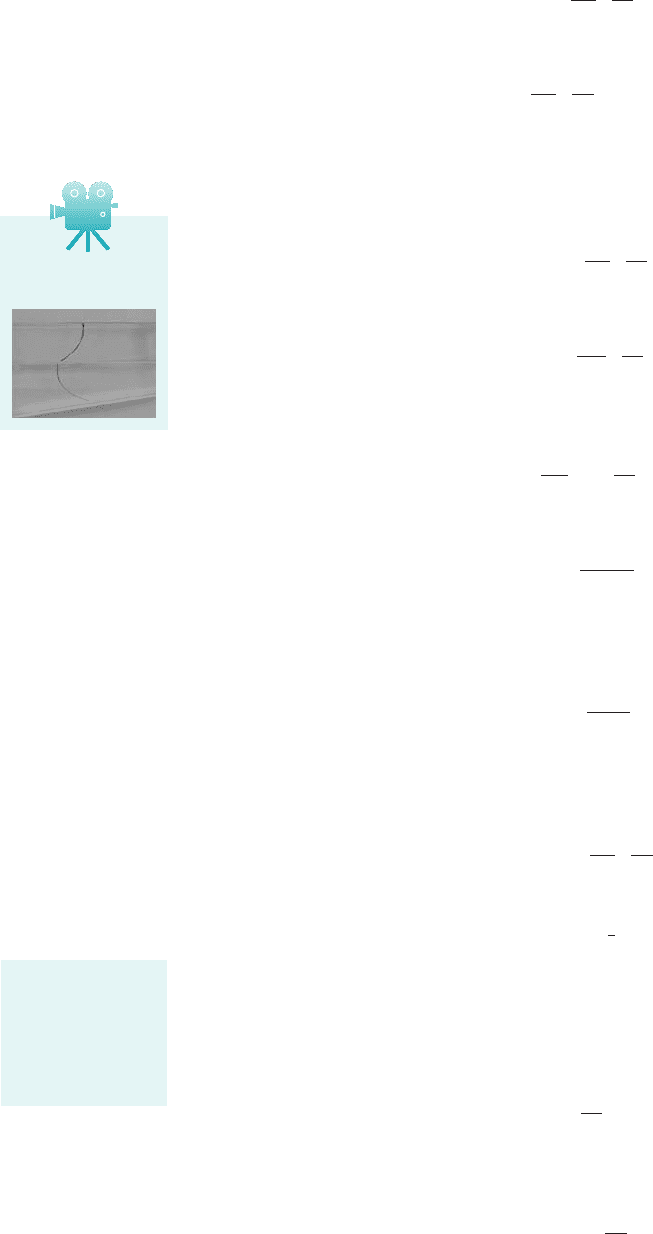
GIVEN A wide moving belt passes through a container of a
viscous liquid. The belt moves vertically upward with a constant
velocity, V
0
, as illustrated in Fig. E6.9a. Because of viscous forces
the belt picks up a film of fluid of thickness h. Gravity tends to
make the fluid drain down the belt. Assume that the flow is lami-
nar, steady, and fully developed.
FIND Use the Navier–Stokes equations to determine an ex-
pression for the average velocity of the fluid film as it is dragged
up the belt.
S
OLUTION
F I G U R E E6.9
a
Plane Couette Flow
This result indicates that the pressure does not vary over a hori-
zontal plane, and since the pressure on the surface of the film
is atmospheric, the pressure throughout the film must be1x h2
y
x
h
Fluid layer
g
V
0
E
XAMPLE 6.9
Since the flow is assumed to be fully developed, the only velocity
component is in the y direction 1the component2so that
It follows from the continuity equation that
and for steady flow so that Under
these conditions the Navier–Stokes equations for the x direction
1Eq. 6.127a2and the z direction 1perpendicular to the paper2
1Eq. 6.127c2simply reduce to
0p
0x
0
0p
0z
0
v v1x2.0v
0t 0,0v
0y 0,
u w 0.
v
JWCL068_ch06_263-331.qxd 9/23/08 12:19 PM Page 312
6.9.3 Steady, Laminar Flow in Circular Tubes
Probably the best known exact solution to the Navier–Stokes equations is for steady, incompressible,
laminar flow through a straight circular tube of constant cross section. This type of flow is commonly
called Hagen–Poiseuille flow, or simply Poiseuille flow. It is named in honor of J. L. Poiseuille 11799–
18692, a French physician, and G. H. L. Hagen 11797–18842, a German hydraulic engineer. Poiseuille
was interested in blood flow through capillaries and deduced experimentally the resistance laws
for laminar flow through circular tubes. Hagen’s investigation of flow in tubes was also
experimental. It was actually after the work of Hagen and Poiseuille that the theoretical results
presented in this section were determined, but their names are commonly associated with the
solution of this problem.
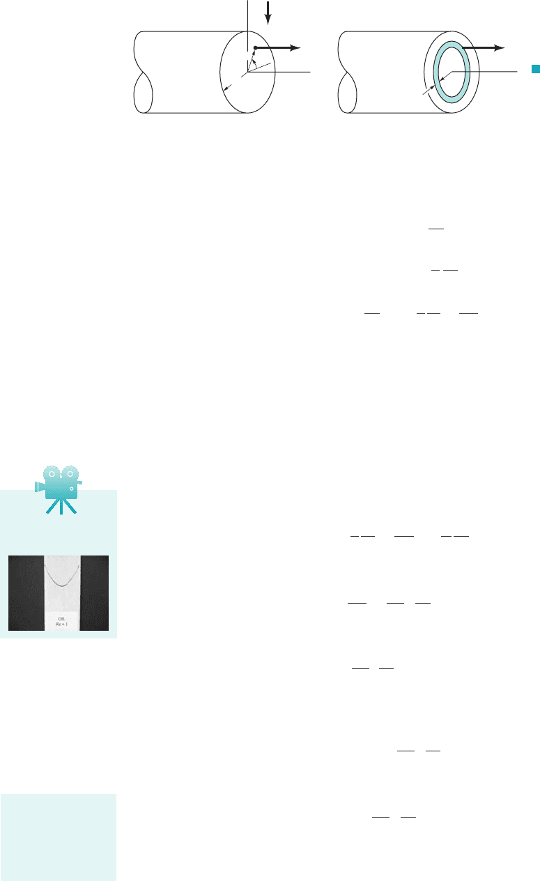
Consider the flow through a horizontal circular tube of radius R as is shown in Fig. 6.34a.
Because of the cylindrical geometry it is convenient to use cylindrical coordinates. We assume that
the flow is parallel to the walls so that and and from the continuity equation 16.342
Also, for steady, axisymmetric flow, is not a function of t or so the velocity, v
z
,uv
z
0v
z
0z 0.
v
u
0,v
r
0
6.9 Some Simple Solutions for Laminar, Viscous, Incompressible Fluids 313
atmospheric 1or zero gage pressure2. The equation of motion in
the y direction 1Eq. 6.127b2thus reduces to
or
(1)
Integration of Eq. 1 yields
(2)
On the film surface we assume the shearing stress is
zero—that is, the drag of the air on the film is negligible. The
shearing stress at the free surface 1or any interior parallel surface2
is designated as , where from Eq. 6.125d
Thus, if at it follows from Eq. 2 that
A second integration of Eq. 2 gives the velocity distribution in
the film as
At the belt the fluid velocity must match the belt velocity,
so that
and the velocity distribution is therefore
(3)
With the velocity distribution known we can determine the
flowrate per unit width, q, from the relationship
q
冮
h
0
v dx
冮
h
0
a
g
2m
x
2
gh
m
x V
0
b dx
v
g
2m
x
2
gh
m
x V
0
c
2
V
0
V
0
,
1x 02
v
g
2m
x
2
gh
m
x c
2
c
1
gh
m
x h,t
xy
0
t
xy
m a
dv
dx
b
t
xy
1x h2
dv
dx
g
m
x c
1
d
2
v
dx
2
g
m
0 rg m
d
2
v
dx
2
and thus
The average film velocity, V is therefore
(Ans)
COMMENT Equation (3) can be written in dimensionless
form as
where c ␥h
2
/2V
0
. This velocity profile is shown in Fig. E6.9b.
Note that even though the belt is moving upward, for c 1 (e.g.,
for fluids with small enough viscosity or with a small enough belt
speed) there are portions of the fluid that flow downward (as in-
dicated by v/V
0
0).
It is interesting to note from this result that there will be a net
upward flow of liquid (positive V) only if V
0
␥h
2
/3. It takes a
relatively large belt speed to lift a small viscosity fluid.
v
V
0
c a
x
h
b
2
2c a
x
h
b 1
V V
0
gh
2
3m
1where q Vh2,
q V
0
h
gh
3
3m
F I G U R E E6.9
b
1
0.8
0.6
0.4
0.2
0
–0.2
–0.4
–0.6
–0.8
–1
c = 2.0
c = 1.0
c = 0
c = 0.5
c = 1.5
0 0.2 0.4 0.6 0.8 1
x/h
v/V
0
An exact solution
can be obtained for
steady, incompress-
ible, laminar flow in
circular tubes.
JWCL068_ch06_263-331.qxd 9/23/08 12:19 PM Page 313
is only a function of the radial position within the tube—that is, Under these conditions
the Navier–Stokes equations 1Eqs. 6.1282reduce to
(6.143)
(6.144)
(6.145)
where we have used the relationships and 1with measured from the
horizontal plane2.
Equations 6.143 and 6.144 can be integrated to give
or
(6.146)
Equation 6.146 indicates that the pressure is hydrostatically distributed at any particular cross
section, and the z component of the pressure gradient, is not a function of r or
The equation of motion in the z direction 1Eq. 6.1452can be written in the form
and integrated 1using the fact that constant2to give
Integrating again we obtain
(6.147)
Since we wish to be finite at the center of the tube it follows that 3since
ln At the wall the velocity must be zero so that
and the velocity distribution becomes
(6.148)
Thus, at any cross section the velocity distribution is parabolic.
To obtain a relationship between the volume rate of flow, Q, passing through the tube and the
pressure gradient, we consider the flow through the differential, washer-shaped ring of Fig. 6.34b.
Since is constant on this ring, the volume rate of flow through the differential area is
dQ v
z
12pr2 dr
dA 12pr2 drv
z
v
z
1
4m
a
0p
0z
b 1r
2
R
2
2
c
2
1
4m
a
0p
0z
b R
2
1r R2102 4.
c
1
01r 02,v
z
v
z
1
4m
a
0p
0z
b r
2
c
1
ln r c
2
r
0v
z
0r
1
2m
a
0p
0z
b r
2
c
1
0p
0z
1
r
0
0r
ar
0v
z
0r
b
1
m
0p
0z
u.0p
0z,
p rgy f
1
1z2
p rg1r sin u2 f
1
1z2
ug
u
g cos ug
r
g sin u
0
0p
0z
m c
1
r
0
0r
ar
0v
z
0r
bd
0 rg cos u
1
r
0p
0u
0 rg sin u
0p
0r
v
z
v
z
1r2.
314 Chapter 6 ■ Differential Analysis of Fluid Flow
y
z
v
z
g
R
r
θ
z
v
z
dr
r
(b)(a)
F I G U R E 6.34
The viscous flow in a horizon-
tal, circular tube: (a) coordi-
nate system and notation used
in analysis; (b) flow through
differential annular ring.
The velocity distri-
bution is parabolic
for steady, laminar
flow in circular
tubes.
V6.13 Laminar
flow
JWCL068_ch06_263-331.qxd 9/23/08 12:19 PM Page 314
and therefore
(6.149)
Equation 6.148 for can be substituted into Eq. 6.149, and the resulting equation integrated to
yield
(6.150)
This relationship can be expressed in terms of the pressure drop, which occurs over a length,
along the tube, since
and therefore
(6.151)
For a given pressure drop per unit length, the volume rate of flow is inversely proportional to the
viscosity and proportional to the tube radius to the fourth power. A doubling of the tube radius
produces a 16-fold increase in flow! Equation 6.151 is commonly called Poiseuille’s law.
In terms of the mean velocity, V, where Eq. 6.151 becomes
(6.152)
The maximum velocity occurs at the center of the tube, where from Eq. 6.148
(6.153)
so that
The velocity distribution, as shown by the figure in the margin, can be written in terms of as
(6.154)
As was true for the similar case of flow between parallel plates 1sometimes referred to as
plane Poiseuille flow2, a very detailed description of the pressure and velocity distribution in
tube flow results from this solution to the Navier–Stokes equations. Numerous experiments
performed to substantiate the theoretical results show that the theory and experiment are in
agreement for the laminar flow of Newtonian fluids in circular tubes or pipes. In general, the
flow remains laminar for Reynolds numbers, below 2100. Turbulent flow in
tubes is considered in Chapter 8.
Re ⫽ rV12R2
Ⲑ
m,
v
z
v
max
⫽ 1 ⫺ a
r
R
b
2
v
max
v
max
⫽ 2V
v
max
⫽⫺
R
2
4m
a
0p
0z
b⫽
R
2
¢p
4m/
v
max
V ⫽
R
2
¢p
8m/
V ⫽ Q
Ⲑ
pR
2
,
Q ⫽
pR
4
¢p
8m/
¢p
/
⫽⫺
0p
0z
/,
¢p,
Q ⫽⫺
pR
4
8m
a
0p
0z
b
v
z
Q ⫽ 2p
冮
R
0
v
z
r dr
6.9 Some Simple Solutions for Laminar, Viscous, Incompressible Fluids 315
Poiseuille’s law re-
lates pressure drop
and flowrate for
steady, laminar flow
in circular tubes.
R
r
v
max
v
z
r
_
R
= 1 –
(
)
2
v
max
V6.14 Complex
pipe flow
Fluids in the News
Poiseuille’s law revisited Poiseuille’s law governing laminar
flow of fluids in tubes has an unusual history. It was developed in
1842 by a French physician, J. L. M. Poiseuille, who was inter-
ested in the flow of blood in capillaries. Poiseuille, through a
series of carefully conducted experiments using water flowing
through very small tubes, arrived at the formula, .
In this formula Q is the flowrate, K an empirical constant, the
pressure drop over the length , and D the tube diameter. Another/
¢p
Q ⫽ K¢p D
4
Ⲑ
/
formula was given for the value of K as a function of the water
temperature. It was not until the concept of viscosity was intro-
duced at a later date that Poiseuille’s law was derived mathe-
matically and the constant K found to be equal to , where
is the fluid viscosity. The experiments by Poiseuille have long
been admired for their accuracy and completeness considering
the laboratory instrumentation available in the mid nineteenth
century.
m
p
Ⲑ
8m
JWCL068_ch06_263-331.qxd 9/23/08 12:19 PM Page 315
6.9.4 Steady, Axial, Laminar Flow in an Annulus
The differential equations 1Eqs. 6.143, 6.144, 6.1452used in the preceding section for flow in
a tube also apply to the axial flow in the annular space between two fixed, concentric cylinders
1Fig. 6.352. Equation 6.147 for the velocity distribution still applies, but for the stationary
annulus the boundary conditions become at and for With these
two conditions the constants and in Eq. 6.147 can be determined and the velocity
distribution becomes
(6.155)
The corresponding volume rate of flow is
or in terms of the pressure drop, in length of the annulus
(6.156)
The velocity at any radial location within the annular space can be obtained from Eq. 6.155.
The maximum velocity occurs at the radius where Thus,
(6.157)
An inspection of this result shows that the maximum velocity does not occur at the midpoint of
the annular space, but rather it occurs nearer the inner cylinder. The specific location depends on
and
These results for flow through an annulus are valid only if the flow is laminar. A criterion
based on the conventional Reynolds number 1which is defined in terms of the tube diameter2cannot
be directly applied to the annulus, since there are really “two” diameters involved. For tube cross
sections other than simple circular tubes it is common practice to use an “effective” diameter,
termed the hydraulic diameter, which is defined as
The wetted perimeter is the perimeter in contact with the fluid. For an annulus
In terms of the hydraulic diameter, the Reynolds number is 1where
area2, and it is commonly assumed that if this Reynolds number remains below
2100 the flow will be laminar. A further discussion of the concept of the hydraulic diameter as it
applies to other noncircular cross sections is given in Section 8.4.3.
cross-sectional
V Q
Re rD
h
V
m
D
h
4p1r
2
o
r
2
i
2
2p1r
o
r
i
2
21r
o
r
i
2
D
h
4 cross-sectional area
wetted perimeter
D
h
,
r
i
.r
o
r
m
c
r
2
o
r
2
i
2 ln1r
o
r
i
2
d
1
2
0v
z
0r 0.r r
m
Q
p¢p
8m/
cr
4
o
r
4
i
1r
2
o
r
2
i
2
2
ln1r
o
r
i
2
d
/¢p,
Q
冮
r
o
r
i
v
z
12pr2 dr
p
8m
a
0p
0z
b cr
4
o
r
4
i
1r
2
o
r
2
i
2
2
ln1r
o
r
i
2
d
v
z
1
4m
a
0p
0z
b cr
2
r
2
o
r
2
i
r
2
o
ln1r
o
r
i
2
ln
r
r
o
d
c
2
c
1
r r
i
.v
z
0r r
o
v
z
0
316 Chapter 6 ■ Differential Analysis of Fluid Flow
v
z
r
i
r
o
z
r
F I G U R E 6.35 The viscous flow through an annulus.
An exact solution
can be obtained for
axial flow in the an-
nular space be-
tween two fixed,
concentric cylin-
ders.
JWCL068_ch06_263-331.qxd 9/23/08 12:20 PM Page 316