Navarra Antonio, Simoncini Valeria. A Guide to Empirical Orthogonal Functions for Climate Data Analysis

Подождите немного. Документ загружается.

3.7 Missing Data 37

possible consequences for EOF analysis as discussed below. The EOF methods

are applied to correlation and covariance matrices. It is tempting to calculate

correlations using the available data for each pair of series, assuming that this gives

the best estimate of the correlation between each series, even if some correlations

are based on a smaller sample than others. However, this approach can lead to prob-

lems with the inversion of the correlation/covariance matrices to derive the EOF

solutions. It is usually best to make all series complete in some way over the analy-

sis period.

Usually, the analyst decides on a ﬁxed analysis period (say, 1961–1990) and de-

cides on the maximum number of missing values that is acceptable for a series to be

included (say, at least 25 out of 30 values must have data). A simple and quite robust

solution to missing data is to set all missing values in a series equal to the mean of

the available data for that series. This will ensure the missing values are all zero

anomalies when the correlation/covariance matrices are calculated. Zero anomalies

have least impact on the correlation/covariances. While it can reduce some genuine

cross correlations between time series and this can distort the EOF solutions, it is

nonetheless a cautious conservative approach and as such, is an attractive solution.

Application of more sophisticated interpolation methods requires care for any in-

crease in correlations/covariances that it may introduce into the datasets.

Chapter 4

Empirical Orthogonal Functions

4.1 Introduction

The atmospheric ﬁelds are three-dimensional ﬁelds by nature, the variation in

longitude, latitude and altitude of winds, temperatures and the other quantities are

normal. A major jump forward in the development of climate science was reached

when it was realized that the analysis of simultaneous values of the variables con-

tained signiﬁcant information. Indeed, to advance scientiﬁc understanding it is

essential to have a view of the relation that links together various climate variables,

for instance the temperature and the pressure in various places.

The covariance matrix is the statistical object that rigorously describes such rela-

tions. Let us consider the case of monthly time series data, for instance temperatures,

for stations in m locations and for a period of n months. Each station can be repre-

sented by a vector, x

D .x

.1/; x

.2/;:::;x

.n//; and the stations can be arranged

in an array;

D Œx

.1/ x

.2/ ::: x

.n/

D Œx

.1/ x

.2/ ::: x

.n/

D Œx

.1/ x

.2/ ::: x

.n/:

Organizing the data in this way suggests an alternative description for the global

data set of station time series. Instead of ordering them as time series, we can order

along the vertical columns. The array we obtain is equivalent to considering vectors

of values at the same time, the so called synoptic view. In mathematical terms we

can treat the array as an m n matrix as follows

X D

.1/ x

.2/ ::: x

.n/

.1/ x

.2/ ::: x

.n/

.1/ x

.2/ ::: x

.n/

; (4.1)

A. Navarra and V. Simoncini, A Guide to Empirical Orthogonal Functions

for Climate Data Analysis, DOI 10.1007/978-90-481-3702-2

 Springer Science+Business Media B.V. 2010

40 4 Empirical Orthogonal Functions

or introducing the synoptic vectors x



D Œx

.j /; x

.j /; : : : ; x

.j / for j D

1;2; :::; nwe have the matrix X deﬁned in terms of column vectors,

X D Œx

; x

; :::; x

;

where the rows of the matrix now describe the values at the same spatial location.

In the analysis of meteorological or climatological data it is very common that

time series come from observations or from numerical simulations taken at reg-

ular intervals. A typical example are for instance temperatures taken at several

stations around the world, grouped in monthly means, so that only one value per

month is available. In this case the columns of the data matrix X indicate the time

series at each station, whereas the synoptic vectors, i.e. the rows of the data ma-

trix, describe the geographic distribution of the temperature at a particular time. The

time evolution of the temperature can then be followed by looking at the sequence

of geographical maps depicting the temperature distribution every month. Usually,

for interpretation purposes it is useful to use contouring algorithms to represent the

ﬁeld as a smooth two-dimensional function. Contouring is not a trivial operation

and especially for observations that are distributed in space with large gaps and far

from being a regular covering of the surface of the Earth, must be done with care.

Sophisticated techniques, known as data assimilation, are employed to make sure

the data sets are put on regular grids in a physically consistent manner. In any case,

either that we are looking at data from modelling, or that we are working with ob-

servations coming from data assimilation systems, we end up with data on regular

grids, covering the Earth with a regular pattern.

As already mentioned, we use two data sets to illustrate our discussion. The ﬁrst

is a time series of monthly mean geopotential data at 500 mb (Z500), obtained from

a simulation with a general circulation model forced by observed values of monthly

mean Sea Surface Temperatures (SST). The data sets cover 34 years, corresponding

to the calendar years 1961–1994. The Z500 set is a very good indicator of upper

air ﬂow, since the horizontal wind is predominantly aligned along the geopotential

isolines. Figure 4.1 shows a few examples taken from the data set. It is possible

to note the large variability from one month to the other (top panels), but also the

large variability at the same point, as the time series for the entire series (lower

panels) show. It is clear that the geopotential at 500 mb is characterized by intense

variability in space and time and a typical month may be as different from the next

month as another one chosen at random.

We can consider the maps at each month as a vector in a special vector space, the

data space. Each vector in this data space represents a map, a possible case of a Z500

monthly mean. The space covers all possible shapes of the Z500, the vast majority

of which will never be realized, like the one in which the heights are constant every-

where, or some other similar strange construction. The mathematical dimension of

This matrix notation is very common in meteorological data, whereas in many other ﬁelds, data

are stored as an n  m matrix, namely as X



. This difference affects the whole notation in later

chapters, when deﬁning the covariance matrix and other statistical quantities.

4.1 Introduction 41

60S

30S

30N

90N

120W 60W

90S

60N

60E 120E 180E

Test data 500mb Geopotential Heights

Test month 1

30S

90N

180E

60N

60W

90S

60S

120W

30N

60E 120E

Test month 2

0 5 10 15 20 25 30 35

–2

Pacific

0 5 10 15 20 25 30 35

−2

Alaska

Fig. 4.1 Examples of Z500 data set. The maps are seasonal means for winter taken from a model

simulation with prescribed Sea Surface Temperatures for a period of 34 years from 1961 to 1994.

Here seasonal anomalies are shown, after removal of the climatological winter mean

the vector space is very high, it is equivalent to the number of observations points, n.

In the case of the test data sets used in this book, which have 96 points along the

longitude for each latitude line and 48 latitude lines, it is n D4608. In fact, this value

42 4 Empirical Orthogonal Functions

is so large that the question arises whether the geopotential in the natural variability

of climate is really exploring all possible combinations of numbers in this 4608 ob-

servation points, in other words the data set we are using may be lying on a subspace

of much smaller dimension.

One question that arises when one is confronted with such an intricate pattern

of behaviors is whether there are special ways in which the Z500 ﬁelds can express

themselves, in other words whether typical recurring patterns exist. In the following

we introduce a possible technique to identify patterns of this kind.

We can gain some insight into the determination of possible subspaces that are

frequently visited if we again consider the data matrix

X D Œx

; x

; :::; x

:

The simplest case of a recurrent pattern subspace occurs if the n vectors are not

linearly independent. In this case, the successive realizations 1,..., n are linear com-

binations of just a few fundamental patterns. The ﬁrst thing to attempt is then to

assess the number of linearly independent columns of X. We have seen in Sect. 2.9

that the rank of X, that is its number of independent columns, may be obtained by

using the SVD. If the rank of X is less than min fm,ng, then some columns will be

just a mixture of the others. The SVD also provides us with a basis for the vector

space spanned by the columns of X (and also for the vector space spanned by the

rows, but we are not interested in that part now) according to X D U†V

: The

decomposition of the data space gives us a mathematical basis for the maps, the

right and left singular vectors, namely the columns of the two matrices V and U.

However, they do not seem to have any special meaning. This is what we will try to

describe in the rest of this chapter.

4.2 Empirical Orthogonal Functions

In the discussion that follows we assume that the data matrix has been transformed

so as to have zero mean vector. This can be easily achieved by subtracting the mean

value to each corresponding row of X,thatisX D X

orig



,where1 is the column

vector of all ones, while

x is the vector of sample means.

With these scaled data, the covariance matrix S can also be written in the follow-

ing way

S D

n 1

: (4.2)

It is easy to check that the combination in (4.2) indeed satisﬁes the deﬁnition of

covariance matrix in (3.2). We can then use the decomposition in singular values of

X that we introduced in the previous section so that

S D U†V

V†U

D U†

: (4.3)

4.3 Computing the EOFs 43

This expression reveals that the left singular vectors of the data matrix X are also

the eigenvectors of the (symmetric) covariance matrix S. We can now understand a

little better the role of the vectors in U. The number of independent maps in the data

sets, the columns of U, are the same as the eigenvectors of the covariance matrix.

Since one is mostly concerned with these modes, which are invariant under scaling

of S, the factor 1=.n  1/ is often omitted when using the covariance matrix S.On

the other hand, care should be taken in working with the eigenvalue diagonal matrix

†

, since scaling S correspondingly scales the eigenvalues.

According to (4.3), the vectors in the unitary matrix U are such that the covari-

ance matrix in that basis is diagonal, that is each vector u is uncorrelated with the

others and contributes to the total variance an amount given by the diagonal element

of †

; indeed, because of the invariance property of the trace, the total variance is

also given by the sum of the squared singular values. Dividing them by the trace we

can get the percentage contribution 

of each mode 





iD1



: (4.4)

If X is not full rank, that is if some of its columns/rows are linearly dependent, then

we will get fewer nonzero singular values, say q, and associated left singular vec-

tors. Equivalently, the covariance matrix has q<minfm; ng nonzero eigenvalues

with corresponding q orthonormal eigenvectors. The independent modes of varia-

tions in U, associated with nonzero singular values, via the SVD of the data matrix,

or via the eigenanalysis of the covariance matrix, are called Empirical Orthogonal

Functions, or in short EOF. Note that in the wide literature on Principal Component

Analysis, these modes are called Principal Components, or PC (see, e.g., Jolliffe

2002).

4.3 Computing the EOFs

The calculation of the eigenpairs of the covariance matrix can be a difﬁcult numer-

ical problem because the dimension of the matrix tends to grow with the number

of observation points. A much faster way to obtain the EOF is to use (4.3)and

perform an SVD on the data matrix. The difference can be of several orders of mag-

nitude in terms of computational cost and it should be considered the right way to

get the EOFs. The SVD decomposition is also more stable and accurate. EOFs can

then be readily computed using M

ATLAB that has primitive functions for both the

SVD and eigenvectors calculation, the former being preferred for computational ef-

ﬁciency (cf. Sect. 4.3.1). As an example, below is a Matlab code that generates all

EOF and projected selected components.

44 4 Empirical Orthogonal Functions

function [u,lam,proj]=eoffast(z,indf,nmode,nproj)

% Compute all EOF of matrix z and expand it for nmode modes

% Also returns nproj projection coefficients

resol = [96 48];

[uu,ss,vv]=svd(z,0); %Memory saving decomposition

lam = diag(ss.ˆ2)/sum(diag(ss.ˆ2)); % Explained variances

u=zeros([resol(1)

resol(2) nmode]);

u(indf,1:nmode)=uu(:,1:nmode);

proj=vv

ss(1:nproj,:)’; % Compute projections

return

For a large matrix, the call to svd in the algorithm above may be replaced by a call

to svds, which computes only a subset of all singular triplets of the given matrix,

as requested by the user. Also in this case, this procedure should be preferred to

the nowadays obsolete strategy of using the power method to compute a few of the

largest eigenvalues of the correlation matrix.

4.3.1 EOF and Variance Explained

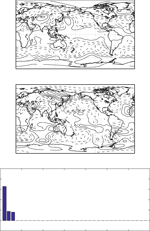
The plots in Fig. 4.2 show the results of performing EOF on a test data set

constructed from the Z500 test set, but in which we have artiﬁcially restricted the

variations to only three independent vectors. An entire data set has then been created

by random combinations of the three. It is possible to see how the EOF has correctly

identiﬁed that there are only three independent vectors.

Following the ratio in (4.4), the three basic modes are contributing to the variance

a fraction that is given in the bottom of Fig. 4.2. The ﬁrst mode is contribut-

ing more than 60% of the variance, whereas the remaining two are more or less

equally dividing the rest. This is somewhat strange since the data set was constructed

by combining the basic vectors with random coefﬁcient uniformly distributed, we

would expect each vector to contribute equally to the variance of the ﬁeld. One hy-

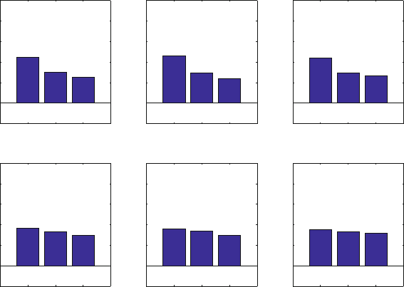
pothesis is that the sample size is too small, but we can see in the subsequent picture

(Fig. 4.3) that increasing the sample size (top row) does not modify the distribution,

and the contribution to the variance remains non-uniform.

The solution to the puzzle must be found in the fact that we have arbitrarily se-

lected the basis vectors. Investigating the vectors it can be found that they are not

mutually orthogonal since their scalar product is not zero. Removing the depen-

dency with an orthogonalization procedure and repeating the analysis we obtain the

bottom row of the ﬁgure. We can see that now each vector contributes uniformly to

4.3 Computing the EOFs 45

0.01

−0.02

0.01

−0.02

0.01

120° W180° E60° E 120° E0° 0°

90° N

60° N

0°

30° N

90° S

60° W

30° S

60° S

Case in which there are only 3 independent maps

EOF 1

0.01

−0.05

−0.02

0.01

0.04

−0.02

120° W180° E60° E

120° E

0° 0°

90° N

60° N

0°

30° N

90° S

60° W

30° S

60° S

EOF 2

0 5 10 15 20 25 30 35

−0.2

0.2

0.4

0.6

0.8

Eigenvalues of the Covariance Matrix

Fig. 4.2 Empirical Orthogonal Functions (EOF) for the test case in which only three independent

maps have been chosen in the Z500 data set and then a complete 34 years set has been reconstructed

with random combination of the three. Here are shown the ﬁrst and the second mode (upper pan-

els) and the spectra of the singular values (lower panels) that reveals that three modes have been

correctly identiﬁed

46 4 Empirical Orthogonal Functions

1 2 3

−0.2

0.2

0.4

0.6

0.8

Variance explained for 50 cases

1 2 3

−0.2

0.2

0.4

0.6

0.8

Variance explained for 100 cases

1 2 3

−0.2

0.2

0.4

0.6

0.8

Variance explained for 500 cases

1 2 3

−0.2

0.2

0.4

0.6

0.8

Variance explained for 50 cases

1 2 3

−0.2

0.2

0.4

0.6

0.8

Variance explained for 100 cases

1 2 3

−0.2

0.2

0.4

0.6

0.8

Variance explained for 500 cases

Fig. 4.3 Variance explained by the three independent modes, in the case of the preceding picture.

The top row shows the variance explained as the sample size increases, passing from 50 to 100

and 500 global maps. The distribution is stable, in fact it is well captured even with 50 cases, but

it is not uniform. In the bottom row we see the variance explained as a function of the sample size

for a test data set in which the basic vector are orthonormalized prior to the generation of the data.

The EOF correctly estimate an equal contribution to the variance, and a modest improvement of

the accuracy can be seen with the increase of the sample size.

the variance as it was expected. In this case the estimation improves with the sample

size as we pass from 50 to 500 cases. This simple experiment leads us to conclude

that the EOF are abstract patterns, that can be used to better (more cheaply) represent

the system total variance. Finally, it is worth noticing that had we used standardized

data, or equivalently the correlation matrix, we would not have observed this in-

triguing phenomenon.

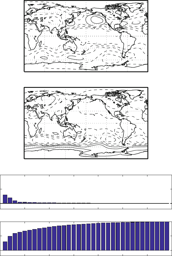
Figure 4.4 shows the EOF for the Z500 data set without any treatment. The mode

patterns are qualitatively similar, but the spectrum is quite different, and it appears

that there are no zero singular values, corresponding to all 34 months being linearly

independent. The interpretation in terms of covariance eigenvectors shows that they

are not all equally important, since we can now rank them according to the size of the

contribution to the total variance. Some vectors give a relatively large contribution

to the variance, whereas others are basically contributing nothing. This means that

this ﬁeld has a preference to vary according to the ﬁrst modes of variations and

consequently the corresponding patterns are most typical.

In general we will obtain as many signiﬁcant EOF as the smallest number be-

tween the length of the time series n and the number of observation points m.

With our test data sets and almost always when treating with climate or weather data,

the number of observation points, either as grid points from simulations or station

4.3 Computing the EOFs 47

0.01

−0.02

90° N

30° N

60° W180° E120° E60° E0° 120° W

60° N

30° S

0°

90° S

0°

60° S

Case in which alla maps are considered

EOF 1

0.01

−0.02

90° N

60° N

0°

60° W120° W120° E

60° E

0° 180° E

30° S

60° S

30° N

0°

90° S

EOF 2

0 5 10 15 20 25 30 35

0.5

Eigenvalues of the Covariance Matrix

0 5 10 15 20 25 30 35

0.5

Cumulative Sum of the Variance Explained

Fig. 4.4 Empirical Orthogonal Functions (EOF) for the Z500 data set. Here are shown the ﬁrst

and the second mode (upper panels) and the singular values (middle panel) that reveals that several

independent modes have been correctly identiﬁed. For instance, the bottom panel illustrates the

cumulative variance explained by the ﬁrst k modes: the ﬁrst ﬁve modes describe together about

60%. The last ten modes have zero contribution