Navarra Antonio, Simoncini Valeria. A Guide to Empirical Orthogonal Functions for Climate Data Analysis

Подождите немного. Документ загружается.

58 4 Empirical Orthogonal Functions

4.5 Reconstruction of the Data

The interpretation of the EOF via the SVD has also another important consequence.

The SVD decomposition of the data matrix

X D U†V



(4.6)

with V D Œv

;:::;v

, can be written in terms of each column of the matrix as

iD1



.k/; q  minfm; ng (4.7)

where we can see that the data can be expressed as a linear combination of the u

vectors, weighted by the singular values (the square root of the variance explained)

and by the kth component of the vectors v. The summation extends to q vectors

depending on the number q of nonzero singular values of X. Equation 4.6 can also be

rearranged to provide the interpretation for the vectors u.WehaveX D U†V



,so

that, multiplying from the left by U



and exploiting the orthogonality of its columns,

we get U



X D †V



. Substituting in (4.7) we obtain for each location vector in

X D Œx

;:::;x

,

D UU



iD1

; x

;kD 1;:::;n: (4.8)

This equation shows that the data can be reconstructed as a linear combination of

the EOF, with coefﬁcients obtained by projecting each data vector onto each EOF.

In this way, the singular value decomposition indicates the minimum number of

vectors that is needed to describe the data space. Individual EOF can still have no

contribution to a certain data map, if the projection of the data vector onto the EOF

is tiny.

Exercises and Problems

1. Consider the matrix of the ﬁrst exercise of Sect. 4.4.3. Show that

X D X  1



can be fully reconstructed as a rank one matrix.

Using the SVD of

X, we can write

X D u

12v



2. Consider the following matrix:

A D U˙V



4.5 Reconstruction of the Data 59

cos 

sin 

sin 

cos 

001

diag.1; 10

3

;10

6

10 0

0 cos 

sin 

0 sin 

cos 



;

with U D Œu

; u

,andV D Œv

; v

 and ˙ D diag.

;

/, 

D =6

and 

D =8. Numerically show that

kA u





D 

; kA u







C 

This result is very general, and provides the error (in the given norm) occurring

in the reconstruction of the given matrix A by means of the ﬁrst few terms in the

SVD.

4.5.1 The Singular Value Distribution and Noise

The set of singular values is sometimes called the spectrum, in analogy with the

spectrum of eigenvalues. We have seen examples of spectra in our constructed case

to show the role of carefully selected data with known composition of the basis

vectors and with known statistics of the data distribution. Reality is much more

complex. Multiple time scales and statistics are present in the data and the problem

is to identify in the total variability the sector of insightful variability where we think

the real physical processes may be at work. The issue is further complicated because

there is no clear and absolute distinction between signal and noise, as the separation

is problem dependent. What is noise for some investigators may be signal for others,

or even for the same investigator at a different time.

The possibility of expanding the data on the EOF that we have seen in the preced-

ing section gives us a very nice opportunity. The results we have obtained are purely

algebraic with no reference to statistics, but the issue of statistics comes in when

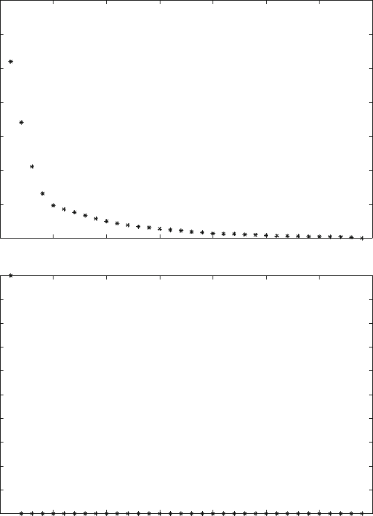
we consider again Fig. 4.12 (the spectra for real Z500). In this case, the spectrum

is similar to the preceding examples, there is a small number of large singular val-

ues, with a long tail of rapidly decreasing values, representing modes that contribute

less and less to the variance. As with all numerical calculations, we have to check

that these values are really non-zero by checking them against the numerical zero of

the calculation. A very useful test for this purpose is to assume that a singular value

of a matrix A is nonzero if

>

; (4.9)

where  is the smallest number represented in the ﬂoating point arithmetic in use (in

ATLAB double precision computation this is 2.2204e-16) and kAk

is the 2-norm

of A (cf. Sect. 2.8), namely its largest singular value. In other words, (4.9)saysthat

the numerical zeros are those values that, when normalized by the largest singular

value, are smaller than the smallest number represented in the employed arithmetic.

A quick inspection reveals that all the sigma’s in Fig. 4.12 pass the test, when the

60 4 Empirical Orthogonal Functions

0 5 10 15 20 25 30 35

0.05

0.1

0.15

0.2

0.25

0.3

0.35

Spectrum of EOF −− Mean Subtracted

0 5 10 15 20 25 30 35

0.1

0.2

0.3

0.4

0.5

0.6

0.7

0.8

0.9

Spectrum of EOF

Fig. 4.12 Singular value distribution for a real case (global Z500 data sets). Top panel: the mean

value of the data is subtracted before calculation of the EOF. Bottom panel: the mean is not re-

moved. Values are normalized with the trace to express explained variance

double precision computation in MATLAB is taken into account, actually they pass

the test very well, with a difference of several orders of magnitude. We have then

eliminated the idea that some of the small sigma’s can in fact be zero, that only the

ﬁnite nature of the computation is preventing from showing up. It is also interesting

to note that in the case we are mostly interested in here, that is for m  n,thereis

4.5 Reconstruction of the Data 61

exactly one zero singular value when the mean is removed, because the subtraction

of the mean reduces the degrees of freedom of the data by one.

The conclusion that we need to retain all modes may in fact be premature. There

is another issue that we need to investigate. We have computed the EOF on the

available data sample, but it is not at all clear how representative of the true EOF

they are. In practice, we have to realize that our computation is only an estimate of

the EOF of the population from which we have extracted a sample, and we need to

investigate how accurate this estimate is. In particular, we need to evaluate the prob-

ability that some of the sigma’s are zero just because of the choice of the members of

the sample. Some sigma’s can really be zero and correspond to degrees of freedom

that do not contribute to the variability of the ﬁeld, but others may appear nonzero

just because of our particular sampling. An EOF analysis is therefore incomplete

without some consideration on the robustness of the results and their sensitivities to

changes in the sampling or in other aspects of the procedure.

The EOF have identiﬁed some patterns corresponding to observation points that

vary together in an organized manner, but each observation point may have variance

that is uncorrelated from other points, from the point of view of the spatial analysis

of variance that is considered noise.

Mathematically the EOF will tend to ﬁt also those components, thus generating a

ﬁctitious pattern. This is one of the reasons that explains why the higher order EOF

have very complex patterns. They try to ﬁt the variance point by point: a desperate

job since it is mostly uncorrelated. This portion of variance is not really interesting,

but we can exploit this property of the EOF, because we can then use it to gener-

ate data that is free of the noise component, simply by reconstructing the data sets

retaining only the higher modes corresponding to covarying modes (cf. Sect. 4.5).

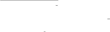
Another example is shown in the following pictures. A two-dimensional wave is

propagating in a square domain from left to right. The wave is a fairly regular sine

wave, but a substantial amount of noise is superposed. At any time the wave pattern

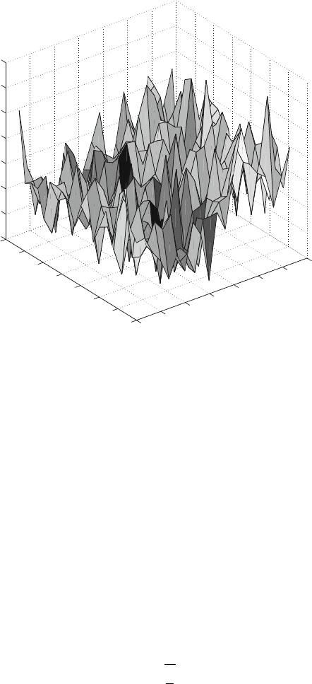
is substantially distorted by the noise (Fig. 4.13). In Fig. 4.14 we display the EOF of

the time evolution, obtained by considering as observation points the local position

at which the wave is observed to pass.

The EOF recover fairly quickly the coherent pattern of the propagating wave

and the ﬁrst two modes explain most of the total variance. We can also see how

propagation is represented by EOF usually employing two modes that are in quadra-

ture and fairly similar in distribution. This indicates that those modes are two phases

of the same propagating pattern. The noise is relegated to higher modes; having

added a signiﬁcant amount of noise, these modes are not insigniﬁcant. The totally

More precisely, using Nx D

X1,wehave

X Nx1



D X.I





Since the matrix I





has rank n 1, the relation above shows that .X Nx1



/ has rank not

greater than minfn  1; mg. Therefore, the scaled covariance matrix .X Nx1



/.X Nx1



has

rank at most n  1,ifm  n.

62 4 Empirical Orthogonal Functions

−30

−20

−10

Fig. 4.13 The propagating wave at an arbitrary instant in the propagation. The average is substan-

tially distorted by the superposed noise

incoherent distribution of these patterns is a very clear indication that in this case

the EOF are trying to ﬁt the individual noise at each observation point.

4.5.2 Stopping Criterion

The division between signal and noise is somewhat arbitrary: how can we decide

when to stop? Though a number of rules to select signiﬁcant EOF have been pro-

posed, their statistical foundation is tenuous. It is better to realize that in practice

the choice is essentially driven by empirical considerations. In the atmospheric lit-

erature, North (North et al. 1982) has proposed the following rule of thumb.He

estimated typical errors using the eigenvalues of the covariance matrix, 

,andthe

number of statistically independent samples in the data







: (4.10)

The rule can then be stated by saying that when the error is larger than or comparable

to the spacing between neighboring eigenvalues, then the sampling error on the EOF

will be comparable to the size of the neighboring EOF. This rule of thumb is often

4.5 Reconstruction of the Data 63

5 10 15 20

Eof 1 0.41973%

5 10 15 20

Eof 2 0.40822%

5 10 15 20

Eof 3 0.012172%

5 10 15 20

Eof 4 0.012051%

5 10 15 20

Eof 5 0.010187%

5 10 15 20

Eof 6 0.0098783%

5 10 15 20

Eof 7 0.0095573%

5 10 15 20

Eof 8 0.0084117%

5 10 15 20

Eof 9 0.0080447%

Fig. 4.14 Empirical orthogonal functions for a propagating wave. The wave propagates from left

to right in the picture. The ﬁrst two modes correspond to the waves, the other modes apparently

try to capture the random noise that had been added to the wave

consistent with another highly employed empirical rule that basically looks for sharp

changes in the convergence to zero of the eigenvalues, the so-called “elbow”. Figure

4.12 shows a sharp change in the curve slope around the ﬁfth and sixth eigenvalues.

64 4 Empirical Orthogonal Functions

The larger eigenvalues are of similar magnitude and they would not pass North’s rule

anyway. The idea is then to retain the eigenvectors before the change and interpret

the others as noise. In practice, there is no objective rule and only the physical

discussion and the identiﬁcation of mechanisms can support the patterns of the EOF

from merely statistical patterns to real physical objects. We refer to Jolliffe (2002),

Quadrelli et al. (2005) for a general thorough presentation of truncation strategies

and error estimation.

From a statistical viewpoint, if the data follow a normal distribution, then it is

possible to formulate an hypothesis test as a stopping strategy. However, in our

context, the condition of normality is often too restrictive to be feasible.

4.6 A Note on the Interpretation of EOF

The technical preparation of the data for analysis and the performance of the EOF

computation themselves may be demanding and time-consuming, to the point that

the original motivations for the work tend to fade. The EOF analysis is just a tool,

and ﬁlling the gap between the EOF modes and the original problem is of major

importance to be able to deduce useful information on the system under analysis.

Interpretation of the EOF is not a form of divination, but it is about connecting

them to the problem. In physical sciences, such an interpretation is often cast in the

form of an “identiﬁcation” of the system physical modes. In more general terms,

EOF may be used to identify recurrent patterns of variations. However, the mathe-

matical nature of EOF generates common mistakes that lead to misinterpretation of

the obtained results.

The main source of the problem lies in the orthogonal nature of the EOF. Or-

thogonality forces a special structure for the modes and sometimes can alter the

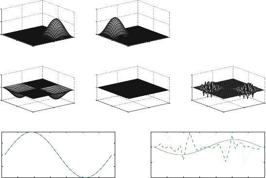
dominant modes quite signiﬁcantly. Figure 4.15 shows an idealized example. Two

modes of variations are set in rectangular domain without overlappingwith the same

amplitude (top panels) as two distinct centers of action. The time variation is given

by another sine wave (bottom left panel). These waves have the same phase so that

they show the same time variation. Each of them represents 50% of the variance in

the data.

The middle panel shows the ﬁrst three EOFs. The ﬁrst EOF shows both centers

together and it explains 100% of the variance, the higher EOF are just noise and

also the time evolution of the EOF coefﬁcients (right bottom panel) shows that the

ﬁrst EOF captures the correct time behavior. This example shows very clearly how

efﬁciently the EOF will capture any co-varying phenomenon, when the center of

actions are separated, but of course does not provide any indication of the causes of

the variations. The EOF aim at maximizing the variance with the smallest possible

number of modes, and this can be done very nicely with only one mode in this

case, but interpreting the ﬁrst EOF mode as the only mode of the system is incorrect

because by construction we had two.

4.6 A Note on the Interpretation of EOF 65

0.5

First Mode -- Variance 50% Second Mode -- Variance 50%

−0.1

0.1

−1

First EOF -- Variance 100% Second EOF -- Variance 0%

−0.2

0.2

Third EOF -- Variance 0%

−1

−0.5

0.5

−1

−0.5

0.5

Time evolution of the physical modes

No Phase Difference

Time evolution of the EOF

Fig. 4.15 An idealized example. Two modes are considered within a rectangular domain with

a simple sine shape with the same amplitude (top panels). The ﬁrst three EOF are shown in the

middle panel. The ﬁrst mode explains 100% of the variance and the remaining modes represent

just noise. The time evolution of the modes is shown in the left bottom panel. The modes are in

phase so that the time plots are exactly on top of each other. The EOF coefﬁcients in time (right

bottom panel) show the correct behavior for the ﬁrst mode, but just noise for the higher modes

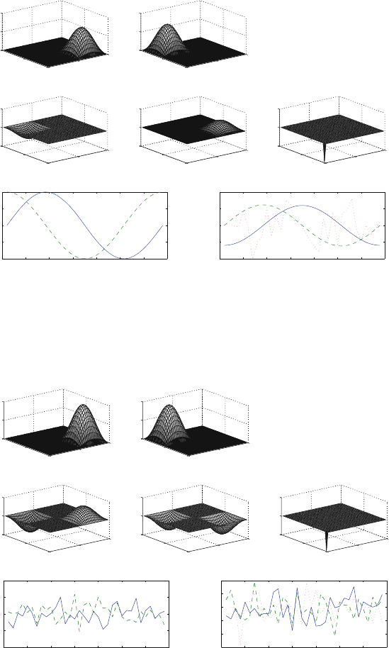
By varying the phase relation in time between the modes the situation changes.

In Fig. 4.16 we have used the same data as in Fig. 4.15, but we have changed the

time phase in a way that the two modes are uncorrelated (bottom left panel). The

variance is split evenly between the modes, except for sampling errors. The EOF

now identiﬁes correctly the existence of two distinct modes; moreover, the estima-

tion of the explained variance is in the right ball park. The higher modes are noise

and they count for a negligible fraction of the variance anyway.

The results for the data in quadrature in time suggest that if the modes are uncor-

related then the EOF can pick them up rather easily. We tried that in Fig. 4.17 where

we assigned as a time evolution random data normally distributed with mean zero

and standard deviation one. In this case the EOF generate two modes that are quite

different from the “modes”. The modes have two centers of action and the ﬁrst one

has the same sign everywhere in the domain; the second must have opposite signs,

so that the overlapping space integral between the two modes is zero, as required by

the orthogonality condition for the EOF. This example is highly inﬂuenced by the

sampling error. The 34 time samples used in this case are simply not sufﬁcient to

correctly identify the independence of the two modes, but it is easy to check that by

increasing the number of time samples the modes are recovered correctly.

66 4 Empirical Orthogonal Functions

Phase Difference π /2

First Mode -- Variance 49% Second Mode -- Variance 51%

0.5

−0.2

0.2

−0.2

0.2

First EOF -- Variance 53%

Second EOF -- Variance 47%

−1

Third EOF -- Variance 0%

0 5 10 15 20

30 35

−1

−0.5

0.5

Time evolution of the physical modes

0 5 10

20 25

−0.4

−0.2

0.2

0.4

Time evolution of the EOF

Fig. 4.16 As in Fig. 4.15 but for the case when the two modes are in quadrature. The time evo-

lution (bottom) shows that they are in quadrature. In this case the EOF modes capture two distinct

modes. The estimation of the variance explained is also good and it will get better as the statistics

is improved

0.5

First Mode -- Variance 48%

0.1

0.2

Second Mode -- Variance 52%

−0.1

0.1

First EOF -- Variance 76%

−0.1

0.1

Second EOF -- Variance 24%

−1

Third EOF -- Variance 0%

5 10

15 20

30 35

−4

−2

Time evolution of the physical modes

Random Phase

0 5 10 15 20

30 35

−0.6

−0.4

−0.2

0.2

0.4

Time evolution of the EOF

Fig. 4.17 As in Fig. 4.15 but for the case when the two modes are uncorrelated in time. The time

evolution (bottom) coefﬁcients are random numbers extracted from a normal distribution with zero

mean and unit standard deviation. In this case the EOF modes capture two distinct modes

4.6 A Note on the Interpretation of EOF 67

0.02

0.04

First Mode

0.5

Second Mode

−0.5

0.5

Third Mode

−0.2

0.2

First EOF -- Variance 68%

−0.2

0.2

Second EOF -- Variance 31%

−0.2

0.2

Third EOF -- Variance 1%

10 15 20 25 30

−2

−1

Time evolution of the physical modes

Overlapping -- Random Phase

0 5 10 15 20 25 30 35

−0.4

−0.2

0.2

0.4

0.6

Time evolution of the EOF

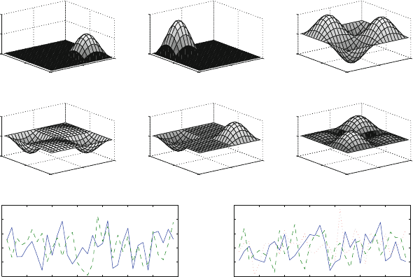
Fig. 4.18 As in Fig. 4.15 but for the case when there are three modes uncorrelated in time. The

time evolution (bottom) coefﬁcients are random numbers extracted from a normal distribution with

zero mean and unit standard deviation. In this case the EOF modes capture two distinct modes

The general picture changes completely in case the analyzed physical modes are

not orthogonal. In Fig. 4.18 we display a situation when we have three modes: the

ﬁrst two modes are the same as the previous examples, but we have added a third

mode that is not localized to only one quarter of the domain but it extends over the

entire domain, overlappingthe other modes. The EOF are shown in the middle panel

and it is clear that they have signiﬁcant deviations from the target modes. Of course

sampling errors are still playing a role, but the main problem here is that the overlap

makes it really hard for the orthogonal EOF to identify the modes.

These examples show that the interpretation of the EOF is often a delicate issue

and it is important to keep in mind that the orthogonality constraint will very easily

generate wave-like patterns, which may be easily misinterpreted as oscillations.

Exercises and Problems

1. Show by Matlab computation how the EOF modes change in Fig. 4.17 if the

sample size is increased.

2. Show by Matlab computation how the EOF modes change in Figs. 4.15–4.17 if

the phase relation between the modes is modiﬁed.