Navarra Antonio, Simoncini Valeria. A Guide to Empirical Orthogonal Functions for Climate Data Analysis
Подождите немного. Документ загружается.


48 4 Empirical Orthogonal Functions
0
0.01
0
0
0
0
0
0
0° 60° W120° W120° E60° E 180° E 0°
0° 60° W120° W120° E60° E 180° E 0°
60° W120° W120° E 180° E 0°
0° 60° W120° W120° E60° E 180° E 0°
0°
60° W120° W120° E60° E
180° E
0°
0°
60° W120° W
120° E
60° E
180° E
0°
90° N
60° N
0°
30° S
60° S
30° N
90° S
90° N
60° N
0°
30° S
60° S
30° N
90° S
90° N
60° N
0°
30° S
60° S
30° N
90° S
90° N
60° N
0°
30° S
60° S
30° N
90° S
90° N
60° N
0°
30° S
60° S
30° N
90° S
90° N
60° N
0°
30° S
60° S
30° N
90° S
EOF Mode 1 29.6%
0.01
0
0
0
0
0
0
0
EOF Mode 2 19.5%
0.01
0.01
0.01
0.01
0.01
0
0
0
0
0
EOF Mode 3 10.1%
0.01
0.01
0.04
0.01
0
.01
0.01
0.01
0
0
0
0
0
0
0
0
0
0
EOF Mode 4 4.2%
0.01
0.01
0.01
0.04
0.01
0.01
0.01
0.01
0
0
0
0
0
0
0
0
0
60° E0°
EOF Mode 5 3.9%
0.01
0.01
0.01
0.01
0.01
0.01
0
0
0
0
0
0
0
0
0
EOF Mode 6 3.3%
EOF
full
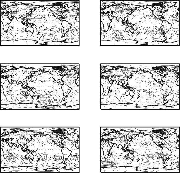
Fig. 4.5 Empirical Orthogonal Functions (EOF) for the Z500 data set. Here are shown the first 6
modes and the amount of variance explained by each mode. The modes have increasingly complex
spatial structures, as it is required by the constraint of orthogonality. The higher modes, shown in
the following pictures, are increasingly disordered. The physical interpretation of the higher modes
is very tricky and it must be done very carefully
data from observations, is always much larger than the length of the time series, that
is m n. In our case we will therefore obtain a maximum of n D 34 EOF. Figure
4.5–4.6 shows the first 12 EOF for the Z500 data. The first three EOF are of course
thesameasthoseinFig.4.4, but the others have more complicated structures. They
present themselves as irregular oscillations in space, with an increasing number of
positive and negative centers. This is to be expected as the orthogonality constraint
with respect to previous EOF forces them to have zero scalar product. We can also
see from the spectrum (Fig. 4.4) that the vast majority of the modes correspond to
very small eigenvalues, contributing very little to the total variance. In fact the cu-
mulative variance expressed by the first m modes (bottom of Fig. 4.4) shows that in
this case the first 15 modes contribute 80% of the variance, and the rest of the vari-
4.4 Sensitivity of EOF Calculation 49
0.01
0.01
0.01
0.01
0.01
0.01
0
0
0
0
0
−0.03
0
0
0
0
60° W180° E60° E 120° E0° 120° W
90° N
60° N
0°
30° N
90° S
0°
60° W180° E60° E
120° E
0° 120° W 0°
60° W180° E60° E
120° E
0° 120° W 0°
60° W180° E60° E 120° E0° 120° W 0°
60° W180° E60° E 120° E0° 120° W 0°
60° W180° E60° E
120° E
0° 120° W 0°
30° S
60° S
90° N
60° N
0°
30° N
90° S
30° S
60° S
90° N
60° N
0°
30° N
90° S
30° S
60° S
90° N
60° N
0°
30° N
90° S
30° S
60° S
90° N
60° N
0°
30° N
90° S
30° S
60° S
90° N
60° N
0°
30° N
90° S
30° S
60° S
EOF Mode 7 3.1%
0.01
0.01
0.01
0.01
0.04
0.01
0.01
0
0
0
0
0
0
0
EOF Mode 8 2.9%
0.01
0.01
0.01
0.01
0
0
0
0
0
−
0.03
0
0
0
0
EOF Mode 9 2.6%
0.01
0.01
0.01
0.01
0
0
0
0
0
−0.03
−0.03
0
0
0
EOF Mode 10 2.4%
0.01
0.01
0.01
0.01
0.01
0
0
0
0
0
−0.03
0
0
0
0
0
EOF Mode 11 2.1%
0.01
0.01
0.01
0.01
0
0
0
0
0
−0.03
0
0
0
0
0
EOF Mode 12 1.8%
EOF
full
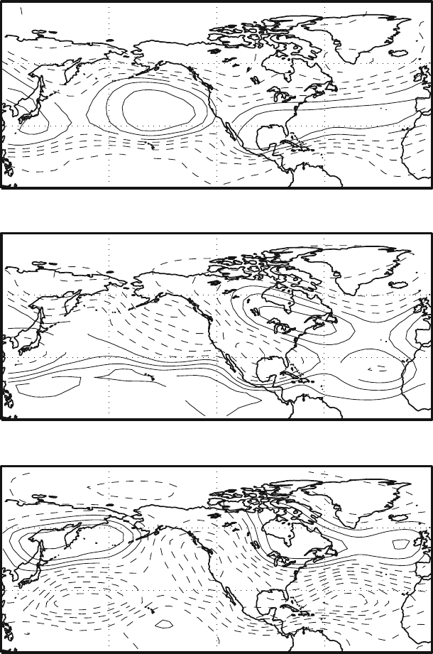
Fig. 4.6 Empirical Orthogonal Functions (EOF) for the Z500 data set. Here are shown the first
7–17 modes and the amount of variance explained by each mode. The modes have increasingly
complex spatial structures, as it is required by the constraint of orthogonality. The higher modes,
shown in the following pictures, are increasingly disordered. The physical interpretation of the
higher modes is very tricky and it must be done very carefully
ance must be attributed to the remaining modes. It is very reasonable to conclude
that these latter modes are not important to describe the overall variance of the field,
whereas the first modes, corresponding to large fractions of contributed variance,
must be of larger relevance.
4.4 Sensitivity of EOF Calculation
We have seen that EOF can be readily calculated, even for large data sets, like the
artificial uniformly distributed data with 500 cases of Fig. 4.3. The interpretation
of the EOF is provided by the terms of variance explained and recurrent patterns,
50 4 Empirical Orthogonal Functions
but if a viable interpretation has to be found, it must rely on a robust determination
of the pattern themselves. The SVD algorithm is robust and reliable algorithm, so
we are not really concerned with mathematical and/or numerical sensitivities, but
with sensitivities deriving from the other possible choices that we can tackle in the
definition of the problem itself. A simple mathematical uncertainty is, for instance,
that eigenvectorsare computed up to a change in sign, as it can be derived from (4.2).
Moreover, data can be normalized in different ways. This operation is often done to
stress one aspect or another of the data, as one may want to consider a different
geographical domain or to analyze a certain area for economy of calculation and
space. In the following we will discuss how the EOF react to this kind of changes.
4.4.1 Normalizing the Data
Data can be normalized in several ways. As we have seen when discussing the
correlation matrix, the most common normalization is the division by the standard
deviation. For the considered multi-variate set this implies dividing by a standard de-
viation that is different for each station. This approach allows us to compare time
series for stations that have large differences in the amplitude of the variability and
focus on the time consistency relation among station time-series. As in previous
sections, in the following we assume that the vector mean has been removed from
the data matrix, so that we can assume that the sample mean is 0. The normalization
of the data can be obtained by dividing each column of the data matrix X in (4.1)by
the standard deviation of each station,
1
;
2
;:::;
m
,thatis
Y D D
1
X
X; with D
X
D diag.
1
; :::;
m
/: (4.5)
We can then proceed to compute EOF on the normalized data matrix Y.Aswe
already observed, the covariance matrix of Y is the correlation matrix of the original
data X. However, by normalizing the original matrix, we can compute the EOF at
once directly using the SVD of Y, without first computing the correlation matrix.
The EOF of Y are sometimes called correlation EOF as opposed to the covari-
ance EOF of the unnormalized data that we have seen in the last section. The main
differences between the two approaches is that the covariance EOF are going to
be biased toward the region of highest standard deviation, so the patterns will try
to optimize as much as possible the variation of the field in those regions. On the
contrary in the correlation EOF, the normalization equalizes the field variations and
so the time series at every station are considered equally important, as a result the
patterns will try to described as much as possible the overall spatial variation of
the field. The standard deviation has a spatial structure (Fig. 4.7) and the effect of
normalization is to reduce the amplitude of the variations in the North Pacific and
North Atlantic, whereas the amplitude is expanded in the other regions.
We show in Figs. 4.8 and 4.9 what happens when computing covariance and cor-
relation EOF on our test data set. The main comment is that the first mode is weakly
4.4 Sensitivity of EOF Calculation 51
25
25
25
25
25
25
50
Test data 500mb Geopotential Heights
Standard Deviation
120E 180E 120W 60W
0
30N
60N
90N
Fig. 4.7 Standard Deviation for the Z500 field
affected, whereas the impact is more noticeable in the higher modes. This is to be
expected: the first mode is expressing the major variance mode, so that large, active
centers of variation will be well represented with or without normalization. But after
the large variations have been removed and higher modes are considered, the impact
of normalization increases as the residual variance is different from one case to the
other. Here, it is possible to see that correlation and covariance EOF convey differ-
ent information and we cannot conclude that there is a preferred method regarding
normalization. Correlation EOF are to be preferred if the investigator is seeking an
overall treatment of all stations, whereas the covariance EOF are simpler to inter-
pret physically, as long as the predominance of the major center of variation is not
an impediment to the investigation. In most cases, the most important patterns will
remain only slightly affected by the change, as in our example.
The effect of the change in normalization becomes progressively larger as we
go up the ladder of modes. This gives some confidence on the reliability of the first
mode, but it may cast some doubts on the other modes; how are we going to interpret
the other modes?
4.4.2 Domain of Definition of the EOF
To analyze the EOF, in the previous discussion we have selected only a portion of the
globe. This is different from the other pictures that represented the entire global data
set. The algebraic tools we have used are valid for any row length m that is, there is
complete freedom in the choice of the number of stations to perform the EOF anal-
52 4 Empirical Orthogonal Functions
120° W120° E 180° E 60° W 0°
60° N
30° N
90° N
0°
0.04
0.04
0.04
0.01
0.01
0.01
0.01
0.01
0
0
0
0
0.01
−0.03
−0.03
−0.03
0
EOF Mode 2 17%
120° W120° E 180° E 60° W 0°
60° N
30° N
90° N
0°
0.01
0.01
0.04
−0.06
0
0
0
0
0.01
0
−0.03
−0.03
−0.03
−0.03
−0.03
0
0.01
0.01
EOF Mode 3 7%
−0.03
0.01
0.01
0.01
0.01
0.01
−0.03
0
0
0
0
0.01
0
−0.03
−0.03
−0.03
−0.03
0
120° W120° E
180° E 60° W
60° N
30° N
90° N
0°
0°
EOF Mode 1 37%
Correlation EOF
Fig. 4.8 Correlation empirical orthogonal functions (EOF) for the Z500 field
4.4 Sensitivity of EOF Calculation 53
0.04
0.04
0.04
0.07
0.1
0.01
0.01
0.01
0.01
0.01
0.01
0
0
0
0
0
−0.03
−0.03
−0.03
0
EOF Mode 1 39%
0.07
0.04
0.01
0.01
0.01
0.01
0.01
0.04
0
0
0
0
0
0.01
−0.03
−0.06
−0.03
−0.03
0
0.01
EOF Mode 2 15%
0.01
0.04
0.04
0.07
−0.09
0
0
0
0
0
0
0.01
0
−0.06
−0.03
−0.03
−0.03
0
0
0
0.01
0.01
0.01
EOF Mode 3 8%
Covariance EOF
120° W120° E
180° E 60° W
60° N
30° N
90° N
0°
120° W120° E
180° E 60° W
0°
120° W120° E
180° E 60° W
0°
0°
60° N
30° N
90° N
0°
60° N
30° N
90° N
0°
Fig. 4.9 Covariance empirical orthogonal functions (EOF) for the Z500 field
54 4 Empirical Orthogonal Functions
ysis. In fact, in terms of the discussion in Sect. 4.1, a different geographical domain
means that a different subset of observation points must be selected. The compu-
tation of the EOF follows the same steps for any number of observation points.
We will obtain patterns that will try to maximize the variance over the new region,
but the optimization of the variance explained is done globally over all stations, so it
is possible that eliminating some station may influence the overall optimization and
hence generate different patterns. Therefore, it is important to determine whether the
obtained patterns are really capturing the major modes of variation we are interested
in, without being overly influenced by far stations.
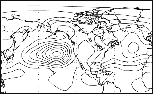
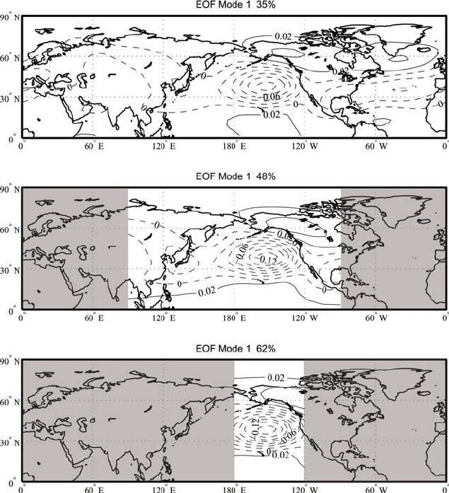
Figure 4.10 shows the result of computing EOF over different geographical do-
mains. The top picture represents the first EOF of the test case for a domain that has
Fig. 4.10 Sensitivity to geographical domain for the Z500 data. The top picture represents the
first EOF for the Northern Hemisphere, the other panels are again the first EOF but excluding the
shaded domain
4.4 Sensitivity of EOF Calculation 55
been already altered from the global domain used previously. We have selected here
the North Hemisphere. Each panel in the picture shows the same first mode com-
puted on smaller and smaller domains. We can see that the EOF are very consistent
from one domain to the next, the computed pattern shape is very similar to each
other and the activity centers are correctly identified in each domain. In this case
we can be confident that the EOF really represent a major mode of variation. On
the other hand, it is interesting to note that the amount of explained variance varies
considerably, more than doubling from the hemispheric case to the smallest domain.
This reflects the fact that as the domain gets smaller the mode becomes more and
more dominant over the total variance in the area and it explains a larger and larger
fraction of the variance.
It is important to keep in mind that the smaller modes of variation are depen-
dent on the geographical domain; what we see here is that we do not get spurious
influences from areas of low variability on the identification of the areas of high
variability. Had we chosen a completely different domain not including the major
center in the Pacific, we would have gotten a completely different mode, because
that mode would explain most of the variance over the new area, unless we attempt
to also explain the variance elsewhere. For instance, the shape over India would have
been different had we chosen a domain only over India.
4.4.3 Statistical Reliability
The EOF computed in previous sections are an estimate. They represent the estimate
of the true modes of variability performed with the particular available sample. It
is very important to give an assessment of the statistical significance of the patterns
that have been found with the method. This is a very active and challenging area
of research since we are dealing with spatial fields and it is actively investigated,
but sometimes a simpler approach can still give a rough idea, that can be used to
identify gross problems. A simple idea is to divide the data sets and repeat the anal-
ysis, aiming to test the statistical robustness to perturbations in the sampling and
distribution of the data. In practice a subset must be defined within the data set and
the EOF analysis must be repeated on the smaller sample. The choice of the sub-
set is of course arbitrary: splitting in two the time series, or sub sampling them in
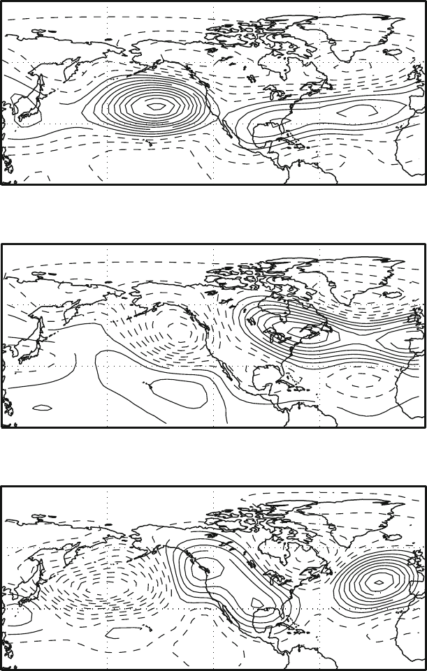
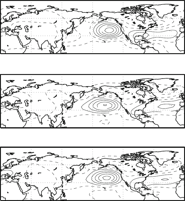
some manner are very popular choices. Figure 4.11 shows what happens when the
EOF are computed on subsets of the original data consisting of the odd and even
years.
The first mode appears rather insensitive to the subsampling, repeating almost
identical in the smaller sets and in the total time series. Though this is not a rigorous
test, it is usually a reasonably good indication of the absence of major problems in
thedatasampling.
56 4 Empirical Orthogonal Functions
0.02
0.02
0.08
0
0
0
0
0
0
0
Odd Years − EOF Mode 1 29%
0.02
0.02
0.02
0.02
0.08
0.02
0
0
0
0
0
0
0
Even Years − EOF Mode 1 40%
0.02
0.02
0.02
0.08
0
0
0
0
0
0
0
Total − EOF Mode 1 33%
Sensitivity to Time Series
60° N
30° N
90° N
0°
60° N
30° N
90° N
0°
60° N
30° N
90° N
0°
60° W
180° E
60° E
120° E
0°
120° W
0°
60° W
180° E
60° E
120° E
0°
120° W 0°
60° W
180° E
60° E
120° E
0°
120° W
0°
Fig. 4.11 Sensitivity to sampling for the Z500 data. The top picture represents the first EOF for
the Northern Hemisphere, selecting only the even years of the data set, the middle panel is the EOF
for the odd years and the bottom panel is for the total
Exercises and Problems
1. Show by Matlab computation that the covariance matrix of the (tall rectangular)
data matrix
X D
0
B
B
B
B
B
@
11 1
102
11 1
102
11 1
1
C
C
C
C
C
A
:

4.4 Sensitivity of EOF Calculation 57
can be obtained both by the command S D cov.X/, as well as by means of the
SVD of X. Comment on the computed EOF.
On the one hand, we obtain
S D cov.X/ D
3
10
0
@
000
013
039
1
A
:
The mean vector of X is
N
x
D Œ1; 0:6; 0:2, so that the zero mean matrix asso-
ciated with X is
b
X D X 1
N
x
D
1
5
0
B
B
B
B
B
@
026
0 3 9
026
0 3 9
026
1
C
C
C
C
C
A
:
The SVD of
b
X, ŒU;˙;V D svd.
b
X/ yields the matrices
V D
1
p
10
0
@
00
p
10
13 0
3 10
1
A
;˙D diag.
p
12;0;0/;
from which, for n D 5, we obtain
1
4
V†
2
V
D S. We observe that the only signif-
icant EOF is given by the scaled version of the vector v D Œ0;1;3
, associated
with the only nonzero singular value.
2. DothesameforthematrixX
. The covariance matrix is
S D cov.X
/ D
0
B
B
B
B
B
@
00000
0
7
3
0
7
3
0
00000
0
7
3
0
7
3
0
00000
1
C
C
C
C
C
A
;
while the SVD of X
1mean.X
/ yields
˙ D diag.
p
28=3; 0; 0; 0; 0/: V D
0
B
B
B
B
B
@
01000
1
p
2
00
1
p
2
0
00100
1
p
2
00
1
p
2
0
00001
1
C
C
C
C
C
A
;
from which the result follows.