Navarra Antonio, Simoncini Valeria. A Guide to Empirical Orthogonal Functions for Climate Data Analysis
Подождите немного. Документ загружается.

140 8 Multiple Linear Regression Methods
0 5 10 15 20
0
5
10
15
20
25
30
nz = 6
A − Significance tested for 1%
Variance of Forced manifold for Z 0.83 %
00
60W120W180W120E
60W120W180W120E
30N
60N
90N
30N
60N
90N
Variance of Free manifold for Z 99 %
000.10.1 0.20.2 0.30.3 0.40.4 0.50.5 0.60.6 0.70.7 0.80.8 0.90.9
1
1
1
1
1
Variance of S
0
0
0.1
0.1
0.2
0.2
0.3
0.3
0.4
0.4
0.5
0.6
0.7
0.1
0.8
0.8
0
0.1
0.9
0.1
1
1
120E 180W 120W 60W
20S
10S
0
10N
20N
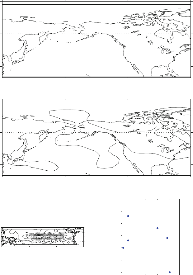
Fig. 8.8 Forced and Free manifolds for the tropical SST, as in Fig. 8.7, including a significance
test and time scrambling the S field. No coherent pattern emerges in the Z field indicating a mostly
casual relation
8.4 The Coupled Manifold 141
8.4 The Coupled Manifold
The analysis of the ensemble experiments with multiple realization showed that the
PRO method is very efficient at identifying the influence of one field on the other, but
this is a somewhat easy case. The presence of multiple cases with the same forcing,
the so-called ensemble, makes it possible to apply other techniques for identifying
the portion of variance that is linked to the external forcing itself. Methods like
separation of variance (Rowell 1997) or even the simple usage of the ensemble
mean can give a good indication of the characteristics of the forced response, even
in case they miss the detailed separation of the time series of the field themselves.
All these approaches however fail when we are confronted with the case of a single
realization.
There are several cases in which executing ensembles is impossible or forbidden
by the terms of the physical problem. In general this can happen when the two
fields that we want to examine are part of the same dynamically linked problem
and they cannot be separated in a “forcing” and a “response”. Coupled atmosphere–
ocean climate simulations are in this class with regard to our examples of marine
temperatures (SST) and atmospheric geopotential Z, since in this case the evolution
of the SST is not prescribed externally but is partially determined by the geopotential
itself. We then have to investigate to what extent the geopotential exerts control over
the SST.
Another notable example are observation records that are not reproducible. In
many cases experiments can be repeated and statistical ensembles can be con-
structed but in geophysical application observations cannot be reproduced in a strict
sense. The Earth atmosphere and ocean constantly evolve and our record of observa-
tions in time is a single realization of the Earth climate. The situation is very similar
to a numerical simulation performed with a coupled atmosphere–ocean model, also
in this case no parameter can be considered “external” and traditional separation of
variance methods fail.
However the formulation of the Forced Manifold is sufficiently general that it
can be used also in the case in which we have a single realization. Nothing in the
formulation we have used in (8.3)or(8.8) is linked to the availability of multiple
realizations. We can set up the problem also for single data sets Z and S. The only
victim is probably the name, since in this case we do not have “forcing” field and
“response” field and calling it “Forced Manifold” does not seem very appropriate.
We can still separate the field in sectors, but now we have a mutual effect of one field
on the other, then the name Coupled Manifold rather Forced Manifold seems more
appropriate. The Free Manifold, instead, maintains its meaning of variance that is
free from the influence of the field under examination.
The results are shown in Fig. 8.9. We present here the results obtained both under
the problem Z D AS and S D BZ. The top line shows the Coupled Manifold for
Z and the corresponding Free Manifold. We can see a familiar pattern of locations
where the variance of Z is highly influenced by the variations of the SST in the
region. The non-local nature of the analysis means that we can conclude only that
the various geographical locations in Z are globally influenced by the entire region
142 8 Multiple Linear Regression Methods
0 5 10 15 20
0
5
10
15
20
nz = 5
Operator A
Coupled Manifold for Z=AS 19 %
0
0.1
0.1
0.1
0.2
0.2
0.2
0.3
0.3
0.4
0.4
0.3
0.2
0.5
0.1
0.4
0.1
0.5
0.2
0.6
0.3
120E 180W 120W 60W 120E 180W 120W 60W
120E 180W 120W 60W 120E 180W 120W 60W
30N
60N
90N
30N
60N
90N
Free Manifold for Z=AS 81 %
00.10.2 4.03.00.5
0.6
0.7
0.7
0.8
0.8
0.8
0.9
0.9
0.7
0.6
0.5
0.6
0.4
0.9
0.9
0.5
0.5
1
0.8
1
1
1
0.3
0.9
1
1
Coupled Manifold for S=BZ 31 %
0
0
0.1
0.1
0.2
0.2
0.3
0.3
0.4
0.4
0.5
0.5
0.10.2
0.1
0.3
0
0.6
0.4
0.1
Free Manifold for S=BZ 69 %
0
0
0.1
0.1
0.2
0.2
0.3
0.3
0.4
0.4
0.5
0.5
0.5
0.6
0.6
0.7
0.7
0.8
0.8
0.9
0.9
0.4
0.6
1
0.7
0.5
0.8
0.6
0.7
0.80.70.60.50.40.30.2
0.1
0
1
1
0.8
0.9
1
0.8
1
20S
10S
0
10N
20N
20S
10S
0
10N
20N
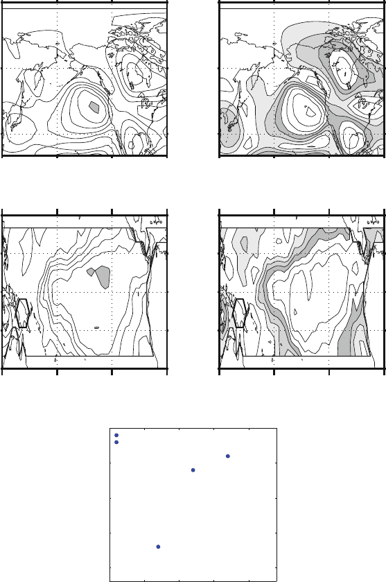
Fig. 8.9 Coupled and Free manifolds for the tropical SST and the North America geopotential.
The significance testing is included. The picture shows the result for the problem Z D AS, top
row, and for the problem S D BZ, bottom row. The significant element of the operator A that is
used in the two problems are shown. Remember that B D A
T
in this calculations. The areas with
a ratio larger than 0.6 are shaded
8.4 The Coupled Manifold 143
in S. The other problem S D BZ gives us the opportunity to see the geographical
distribution of the influence of the entire Z region over the SST variability. We are
looking here at distant regions that show very well the flexibility of these methods:
they can be applied to varying field with few limitations in space and time, but they
must be interpreted with caution.
These methods identify patterns of co-variation that may or may not correspond
to physical causal relation between the fields. For instance, we have theoretical ar-
guments to expect the influence by the tropical SST on the geopotential in the North
America sector and the methods very nicely allow us to investigate this relation
in detail. The opposite formulation makes it possible to investigate instead the in-
fluence of the geopotential Z on the tropical SST and to inspect its geographical
distribution. Unfortunately, in this case we do not have a theory for the influence of
the American geopotential on the tropical SST, so what we see here is basically a
representation of the co-variation relations observed in the previous Z D AS case.
These methods cannot really provide us with causal relation, but they can point us to
the right direction. Only our scientific ingenuity and arguments can then transform
them into cause–effect theories.
The situation may change if we analyze fields where we know on physical
grounds that some interaction is present and therefore some mutual influence ex-
ists. We will expand here slightly our data base extending the test case to a time
series of monthly means of SST and the east–west component of the surface winds,
expressed here as wind stress. The data have been obtained from a long simulation
with a coupled model at low resolution and extended for 200 years.
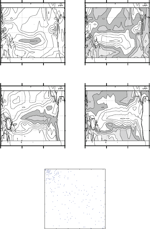
The results shown in Fig. 8.10 indicate a different result from the preceding one.
We know that SST and this component of the surface Wind are strongly interacting
in this region, and we have selected the same geographical domain for the two fields.
The distribution of the Coupled Manifold is consistent with each other as we may
expect in a situation where the two fields exert a mutual influence on each other. The
fraction of variance in the Coupled Manifold is locally very high and values of 70%
are reached. The joint variability region is mostly limited to the equatorial Pacific
and it becomes weaker moving to the higher latitudes.
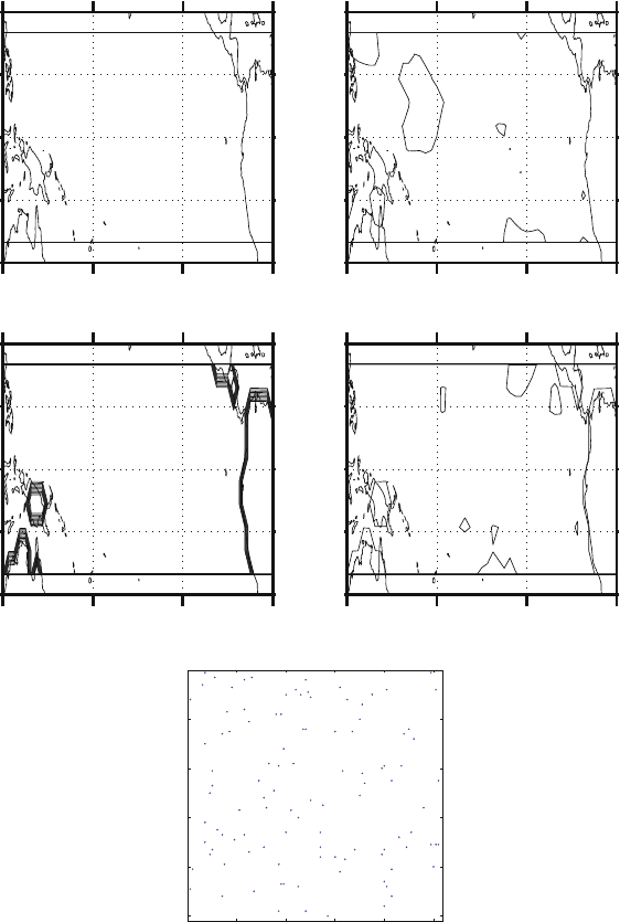
A random permutation of the time series of SST (Fig. 8.11) completely destroys
the relation. The Coupled manifold disappears except for a small residue. The ef-
fect is more dramatic than in the previous scrambling example using SST and the
geopotential; the larger response is due to the stronger couplings that exist between
the SST and the wind and also to the longer time series. The latter is what makes
the relation between the fields more accurate.
These results are quite general and they are not limited to this atmosphere-ocean
example. In general longer time series will improve the accuracy and the reliability
of the identification of the relation.
144 8 Multiple Linear Regression Methods
0 20 40 60 80 100
0
20
40
60
80
100
nz = 188
Operator A
Coupled Manifold for Wind, Z=AS 35 %
0
0
0.1
0.1
0.2
0.2
0.3
0.3
0.3
0.4
0.4
0.5
0.5
0.6
0.4
0.3
0.2
0.4
0.4
0.5
0.5
0.6
0.2
0.2
0.4
0.6
0.4
0.7
120E 180W 120W 60W
120E 180W 120W 60W 120E 180W 120W 60W
120E 180W 120W 60W
20S
10S
0
10N
20N
20S
10S
0
10N
20N
20S
10S
0
10N
20N
20S
10S
0
10N
20N
Free Manifold for Wind, Z=AS 65 %
0
0
0.1
0.1
0.2
0.2
0.3
0.3
0.4
0.4
0.5
0.5
0.6
0.6
0.6
0.6
0.7
0.7
0.5
0.8
0.4
0.7
0.7
0.6
0.8
0.8
0.7
0.7
0.5
0.7
0.8
0.3
0.4
0.8
0.9
Coupled Manifold for S=BZ 35 %
0
0
0.1
0.1
0.2
0.2
0.3
0.3
0.4
0.4
0.5
0.5
0.6
0.6
0.7
0.80.9
1
0.4
0.7
0.6
0.3
0.4
0.5
0.6
0.7
0.8
0.9
0.7
1
0.8
0.9
0.6
1
0.7
0.8
0.9
1
0.5
0.3
0.6
0.2
0.3
0.40.5
0.6
0.60.7
0.8
1
Free Manifold for S=BZ 65 %
0
0
0.1
0.1
0.2
0.2
0.3
0.3
0.3
0.4
0.4
0.4
0.5
0.5
0.6
0.6
0.6
0.7
0.7
0.8
0.7
0.8
0.9
1
0.7
0.7
0.8
0.9
1
0.9
1
0.9
1
0.8
0.9
0.9
0.5
0.9
0.7
1
0.2
Fig. 8.10 Coupled and Free manifolds for the tropical SST and surface east–west Wind in the
same region. Significance testing at 1% is included. The picture shows the result for the problem
Z D AS, top row, and for the problem S D BZ, bottom row. The significant element of the
operator A that is used in the two problems are shown. The areas with a ratio larger than 0.6 are
shaded
8.4 The Coupled Manifold 145
0 20 40 60 80 100
0
20
40
60
80
100
nz = 106
Operator A
Variance of Coupled Manifold for Wind 5.5 %
0
0
120E 180W 120W 60W
120E 180W 120W 60W 120E 180W 120W 60W
120E 180W 120W 60W
20S
10S
0
10N
20N
20S
10S
0
10N
20N
20S
10S
0
10N
20N
20S
10S
0
10N
20N
Variance of Free Manifold for Wind 95 %
0
0
0.1
0.1
0.2
0.2
0.3
0.3
0.4
0.4
0.5
0.5
0.6
0.6
0.7
0.7
0.8
0.8
0.9
0.9
0.9
1
1
0.9
1
1
1
Variance of Coupled Manifold for S 4.5 %
0
0
0.1
0.2
0.3
0.4
0.5
0.6
0.7
0.8
0.9
1
0.1
0.2
0.1
0.3
0.2
0.4
0.5
0.1
0.3
0.6
0.2
0.4
0.7
0.3
0.5
0.8
0.4
0.9
0.6
0.5
1
0.6
0.7
0.7
0.8
0.8
0.9
1
1
1
1
Variance of Free Manifold for S 96 %
0
0
0.1
0.1
0.2
0.2
0.3
0.3
0.4
0.4
0.5
0.5
0.6
0.6
0.7
0.7
0.8
0.8
0.9
0.9
1
1
1
1
1
0.9
1
1
Fig. 8.11 Coupled and Free manifolds for the tropical SST and surface east–west Wind in the
same region with a time scrambling of the SST time series. The significance testing is included.
The picture shows the result for the problem Z D AS, top row, and for the problem S D BZ,
bottom row. The significant element of the operator A that is used in the two problems are shown.
The areas with a ratio larger than 0.6 are shaded
146 8 Multiple Linear Regression Methods
Exercises and Problems
1. Using the data sets and the scripts provided compute the EOF of Z
S
and Z
free
and
check that they are different.
2. Show that the elements of A are regression coefficients and that they coincide
with correlation coefficients if the variance scaling is used.
3. Try to compute the Forced and Coupled Manifolds for different regions.
4. Modify the significance settings in the calculation and check how the ratio be-
tween the Forced and Free parts is modified.
5. Show that each field can be expressed as the sum of three terms, using the oper-
ators AB.
References
Barnett TP, Preisendorfer RW (1987) Origins and levels of monthly and seasonal forecast skill for
united states surface air temperatures determined by canonical correlation analysis. Mon Wea
Rev 115:1825–1850
Bretherton CS, Smith C, Wallace JM (1992) An intercomparison of methods for finding coupled
patterns in climate data. J Climate 5:541–560
Cherry S (1996) Singular value decomposition and canonical correlation. J Climate 9:2003–2009
Cherry S (1997) Some comments on the singular value decomposition. J Climate 10:1759–1761
Clarke GM, Cooke D (1998) A basic course in statistics, 4th edn. Arnold, London and New York
Golub H Gene, Charles F Van Loan (1996) Matrix computations, 3rd edn. The John Hopkins
University Press, Baltimore
Hahn SL (1996) Hilbert transforms in signal processing. Artech House, Norwood, Maryland
Harman HH (1976) Modern factor analysis, 3rd edn. University of Chicago Press, Chicago
Horn RA, Johnson CR (1991) Topics in matrix analysis. Cambridge University Press, Cambridge
Jolliffe IT (2002) Principal component analysis, 2nd edn. Springer Series in Statistics, Springer,
New York
matlab7 (September 2004) MATLAB 7. The MathWorks, Inc
Meyer CD (2000) Matrix analysis and applied linear algebra. SIAM, Philadelphia
Navarra A, Tribbia J (2005) The coupled manifold. J Atmos Sci 62:310–330
North GR, Bell TL, Cahalan RF (1982) Sampling errors in the estimation of empirical orthogonal
functions. Mon Wea Rev 110:699–706
Preisendorfer RW (1988) Principal component analysis in meteorology and oceanography, vol 17,
Development in atmospheric sciences. Elsevier, Amsterdam
Roberta Q, Christopher SB, John M Wallace (September 2005) On sampling errors in empirical
orthogonal functions. J Climate 18(17):3704–3710
http://dx.doi.org/10.1175/%2FJCLI3500.1
Richman MB, Vermette SJ (1993) The use of procrustes target analysis to discriminate dominant
source regions of fine sulfur in the western USA. Atm Environ 27A:475–481
Rowell DP (1997) Using an ensemble of multi-decadal gcm simulations to assess potential sea-
sonal predictability. J Climate 11:109–120
von Storch H, Zwiers FW (1999) Statistical analysis in climate research. Cambridge University
Press, Cambridge
Wilks S Daniel (2005) Statistical methods in the atmospheric sciences, 2nd edn. International
Geophysics series, Academic Press, Oxford
147
Index
C
Canonical Correlation Analysis, 107
Barnett–Preisendorfer, 114
CCA, 107
Barnett–Preisendorfer, 114
modes, 118
data reconstruction, 109
explained variance, 109, 112
modes, 111
patterns, 109
time coefficients, 113
CCA-BP, 114
CEOF, 87
climate anomaly, 27
Combined EOF, 90
autocovariance, 94
covariance matrix, 92
crosscovariance, 94
data matrix, 92
normalization, 92
Complex EOF, 86–88
complex EOF, 79, 83
Hilbert transform, 82
imaginary part, 87
real part, 87
contours, 40
correlation coefficient, 30
correlation matrix, 31
covariance coefficient, 30
D
data
matrix, 39
monthly means, 40
noise, 61
normalization, 50
oscillations, 79
propagation, 81
reconstruction, 58
SST, 40
synoptic vectors, 40
Z500, 40
data matrix, 42
E
EEOF, 87
lags, 89
eigenvalue, 17
multiplicity, 17
eigenvector, 17
Empirical Orthogonal Functions, 42
EOF,
42
correlation, 50
covariance, 50
domain definition, 51
filter, 115
filtering, 59
noise, 61
orthogonal, 69
projection, 58
reconstruction, 58
rotated, 70
sensitivity, 55
spatial dependence, 55
spectrum, 59
subsampling, 55
Euclidean
norm, 7
Extended EOF, 87
lags, 89
F
Frobenius norm, 15
functions of matrices, 21
149
150 Index
G
Gram-Schmidt process, 11, 12
H
Hilbert transform, 82
L
linear
combination, 10
dependence, 10
independence, 10
system of unknowns, 16
linear system, 16
M
manifold, 124, 129, 141, 143
Coupled, 141, 143
Forced, 124, 129
Free, 124, 129, 141, 143
matrix, 12
commuting, 15
covariance, 39
diagonal, 14
eigenvalue, 17
eigenvector, 17
functions, 21
Hermitian adjoint, 13
inverse, 13, 16
least squares, 124
normal, 13
null space, 14
orthogonal, 13
polynomial, 21
pseudoinverse, 20, 124
rank, 16, 19
singular, 13, 16
singular values, 19
singular vectors, 19
spectrum, 17
SVD, 19
trace, 15
transpose, 12
triangular, 14
unitary, 13
mean, 27
N
norm
Euclidean, 19
Frobenius, 20, 78
normal distribution, 32
null hypothesis, 32
O
oblique patterns, 79
orthogonal basis, 11
P
Procrustes problem, 128
PROMAX, 79
propagating signal, 83
pseudo-inverse, 20
Q
quadrature, 81
quarter wavelength shift, 82
R
range, 14
rank, 16
regression, 123
multiple, 123
Rotated EOF, 70
explained variance, 74
non-orthogonal rotation, 77
orthogonal rotation, 72
Procrustes problem, 78
PROMAX, 78, 79
VARIMAX, 72, 79
row rank, 107
S
scalar product, 6
scatter plot, 29
separation of variance, 141
similarity transformation, 18
simple pattern, 71
simple structure, 71
Singular Value Decomposition, 19
singular vector
left, 43
singular vectors, 19
speudoinverse, 124
standard deviation, 28
standard error, 33
standardized variable, 28
stationary signal, 83
SVD, 42, 43,
50, 109
economy size, 108