Neubauer A., Freudenberger J., Kuhn V. Coding theory: algorithms, architectures and applications

Подождите немного. Документ загружается.

226 SPACE–TIME CODES

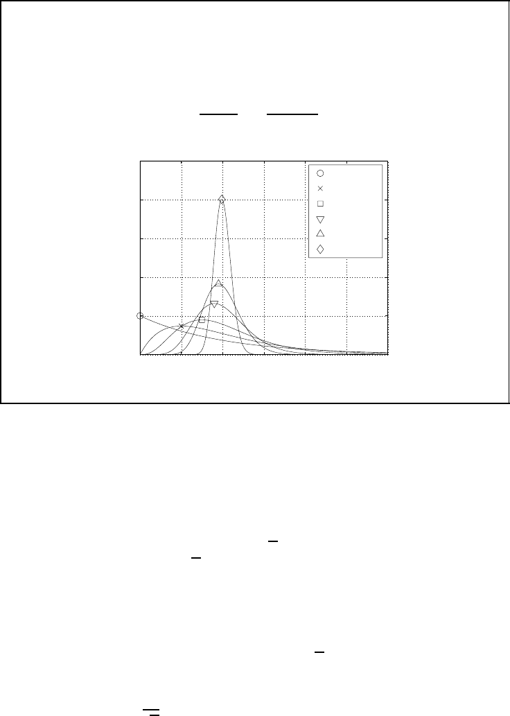
SNR distribution for diversity reception

■ Probability density function of SNR normalised to unit mean

p(ξ) =

D−1

(D − 1)!

· e

−ξD/(E

)

(5.18)

0 0.5 1 1.5 2 2.5 3

ξ →

p(ξ) →

D = 1

D = 2

D = 4

D = 10

D = 20

D = 100

Figure 5.9: Probability density function of SNR for D-fold diversity, Rayleigh

distributed coefﬁcients and Maximum Ratio Combining (MRC). Reproduced by

permission of John Wiley & Sons, Ltd

the expectation with respect to the chi-square distribution with 2D degrees of freedom

has to be determined. For BPSK and i.i.d. diversity branches, an exact solution is given in

Equation (5.21) (Proakis, 2001). The parameter

γ denotes the average SNR in each branch.

A well-known approximation for

γ 1 provides a better illustration of the result. In this

case, (1 + α)/2 ≈ 1 holds and the sum in Equation (5.21) becomes

D−1



=0



D − 1 +







2D − 1



(5.19)

Furthermore, the Taylor series yields (1 − α)/2 ≈ 1/(4

γ). With these results, the symbol

error rate can be approximated for large signal-to-noise ratios by

≈



4γ





2D − 1



(

)

−D



2D − 1



(5.20)

Obviously, P

is proportional to the Dth power of the reciprocal signal-to-noise ratio. Since

error rate curves are scaled logarithmically, their slope will be dominated by the diversity

SPACE–TIME CODES 227

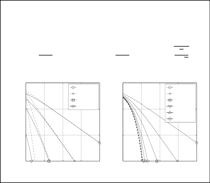
Error rate performance for diversity reception

■ Error probability for Binary Phase Shift Keying (BPSK), Rayleigh density

and D-fold diversity



1 − α



D−1



=0



D − 1 +







1 + α





with α =



1 + γ

(5.21)

0 10 20 30 40

Ŧ6

Ŧ4

Ŧ2

0 10 20 30 40

Ŧ6

Ŧ4

Ŧ2

in dB →

→

D = 1D = 1

D = 2D = 2

D = 4

D = 10

D = 20

D = 100

(a) SNR per antenna

(b) SNR per symbol

in dB →

Figure 5.10: Error probability for D-fold diversity, BPSK, Rayleigh distributed

coefﬁcients and MRC: (a) SNR measured per receive antenna (dashed lines =

approximation from expression (5.20)), (b) SNR per combined symbol (bold dashed line

= AWGN reference)

degree D at high SNRs. This is conﬁrmed by the results depicted in Figure 5.10. In diagram

(a) the symbol error probability is plotted versus the signal-to-noise ratio E

per receive

antenna. Hence, we observe the array gain as well as the diversity gain. The array gain

amounts to 3 dB if D is doubled, e.g. from D = 1toD = 2. The additional gap is caused

by the diversity gain. It can be illuminated by the curves’ slopes at high SNRs, as indicated

by the dashed lines.

In diagram (b), the same error probabilities are plotted versus the SNR after the com-

biner. Therefore, the array gain is invisible and only the diversity gain can be observed.

The gains are largest at high signal-to-noise ratios and if the diversity degree increases

from a low level. Asymptotically for D →∞, the AWGN performance without any fading

is reached.

228 SPACE–TIME CODES

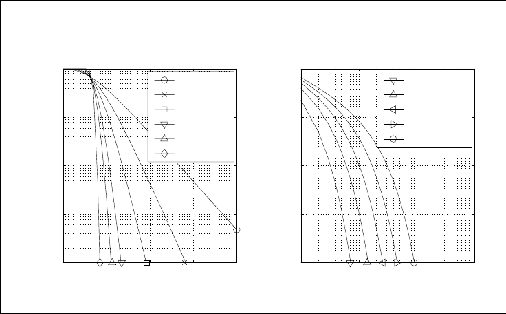
Outage probability

For slowly fading channels, the average error probability is often of minor interest. Instead,

operators are particularly interested in the probability that the system will not be able to

guarantee a speciﬁed target error rate. This probability is called the outage probability P

out

Since the instantaneous error probability P

(γ []) depends directly on the actual signal-to-

noise ratio γ [], the probability of an outage event when maximum ratio combining i.i.d.

diversity paths is obtained by integrating the distribution in Equation (5.17)

out

= Pr{P

(γ [])>P

p(ξ) dξ (5.22)

The target SNR γ

corresponds to the desired error probability P

= P

(γ

). Figure 5.11

shows numerical results for BPSK. The left-hand diagram shows P

out

versus E

for a

ﬁxed target error rate of P

= 10

−3

. Obviously, P

out

decreases with growing signal-to-noise

ratio as well as with increasing diversity degree D. At very small values of E

,we

observe the astonishing effect that high diversity degrees provide a worse performance.

This can be explained by the fact that the variations in γ [] become very small for large

D. As a consequence, instantaneous signal-to-noise ratios lying above the average E

occur less frequently than for low D, resulting in the described effect. Diagram (b) shows

Outage probabilities for diversity reception

0 10 20 30 40

Ŧ4

Ŧ3

Ŧ2

Ŧ1

Ŧ8

Ŧ6

Ŧ4

Ŧ2

in dB →

out

→

out

→

D →

D = 1

D = 2

D = 4

D = 10

D = 20

D = 100

= 10

−1

= 10

−2

= 10

−3

= 10

−4

= 10

−5

(a) P

= 10

−3

(b) 10 log

) = 12 dB

Figure 5.11: Outage probabilities for BPSK and i.i.d. Rayleigh fading channels:

(a) a target error rate of P

= 10

−3

and (b) 10 log

) = 12 dB. Reproduced by

permission of John Wiley & Sons, Ltd

SPACE–TIME CODES 229

the results for a ﬁxed value 10 log

) = 12 dB. Obviously, diversity can reduce the

outage probability remarkably.

5.2 Spatial Channels

5.2.1 Basic Description

Contrary to scalar channels with a single input and a single output introduced in Chapter 1,

spatial channels resulting from the deployment of multiple transmit and receive antennas

are vector channels with an additional degree of freedom, namely the spatial dimension.

A general scenario is depicted in Figure 5.12. It illustrates a two-dimensional view that

considers only the azimuth but not the elevation. For the scope of this chapter, this two-

dimensional approach is sufﬁcient and will be used in the subsequent description. An

extension to a truly three-dimensional spatial model is straightforward and differs only by

an additional parameter, the elevation angle.

As shown in Figure 5.12, the azimuth angle θ

denotes the DoA of an impinging

waveform with respect to the orientation of the antenna array. Equivalently, θ

represents

Channel with multiple transmit and receive antennas

Simple model with discrete DoAs and DoDs:

transmitter

receiver

scatterer

scatterers

T,1

T,2

T,LoS

R,1

R,2

R,LoS

■ Multiple direction of arrivals (DoAs) θ

R,µ

at receiver.

■ Direction of departure (DoD) θ

T,µ

at transmitter depends on Direction of

Arrival (DoA) θ

R,µ

⇒ Channel impulse response h(t,τ,θR) is a three-dimensional function.

Figure 5.12: Channel with multiple transmit and receive antennas

230 SPACE–TIME CODES

the DoD of a waveform leaving the transmitting antenna array. Obviously, both angles

depend on the orientation of the antenna arrays at transmitter and receiver as well as on the

location of the scatterers. For the purpose of this book it is sufﬁcient to presuppose a one-

to-one correspondence between θ

and θ

. In this case, the DoD is a function of the DoA

and the channel impulse response has to be parameterised by only one additional param-

eter, the azimuth angle θ

. Hence, the generally time-varying channel impulse response

h(t, τ ) known from Chapter 1 is extended by a third parameter, the direction of arrival θ

Therefore, the augmented channel impulse response h(t,τ,θ

) bears information about the

angular power distribution.

Principally, Line of Sight (LoS) and non-line of sight (NLoS) scenarios are distin-

guished. In Figure 5.12, an LoS path with azimuth angles θ

T,LoS

and θ

R,LoS

exists. Those

paths are mainly modelled by a Ricean fading process and occur for rural outdoor areas.

NLoS scenarios typically occur in indoor environments and urban areas with rich scatter-

ing, and the corresponding channel coefﬁcients are generally modelled as Rayleigh fading

processes.

Statistical Characterisation

As the spatial channel represents a stochastic process, we can follow the derivation in

Chapter 1 and describe it by statistical means. According to Figure 5.13, we start with the

autocorrelation function φ

(t,τ,θ

) of h(t,τ,θ

) which depends on three parameters,

the temporal shift t, the delay τ and the DoA θ

. Performing a Fourier transformation with

respect to t delivers the three-dimensional Doppler delay-angle scattering function deﬁned

in Equation (5.24) (Paulraj et al., 2003). It describes the power distribution with respect

to its three parameters. If 

,τ,θ

) is narrow, the angular spread is small, while a

broad function with signiﬁcant contributions over the whole range −π<θ

≤ π indicates

a rather diffuse scattering environment. Hence, we can distinguish between space-selective

and non-selective environments.

Similarly to scalar channels, integrations over undesired variables deliver marginal

spectra. As an example, the delay-angle scattering function is shown in Equation (5.25).

Similarly, we obtain the power Doppler spectrum



) =

−π

∞



,τ,θ

)dτ dθ

the power delay proﬁle



(τ ) =

−π



(τ, θ

)dθ

or the power azimuth spectrum



(θ) =

∞



(τ, θ) dτ .

In order to simplify notation, we will use in this subsection a channel representation assuming that all

parameters are continuously distributed.

SPACE–TIME CODES 231

Statistical description of spatial channels

■ Extended channel impulse response h(t,τ,θ

■ Autocorrelation function of h(t,τ,θ

)

(t,τ,θ

) =

∞

−∞

h(t,τ,θ

) · h

∗

(t +t,τ,θ

)dt (5.23)

■ Doppler delay-angle scattering function



,τ,θ

) =

∞

−∞

(ξ,τ,θ

) · e

−j2πf

dξ (5.24)

■ Delay-angle scattering function



(τ, θ

) =

d max

−f

d max



,τ,θ

)df

(5.25)

Figure 5.13: Statistical description of spatial channels

Typical Scenarios

Looking for typical propagation conditions, some classiﬁcations can be made. First, outdoor

and indoor environments have to be distinguished. While indoor channels are often affected

by rich scattering environments with low mobility, the outdoor case shows a larger variety

of different propagation conditions. Here, macro-, micro- and picocells in cellular networks

show a signiﬁcantly different behaviour. Besides different cell sizes, these cases also differ

as regards the number and spatial distribution of scatterers, mobile users and the position of

the base station or access point. At this point, we will not give a comprehensive overview of

all possible scenarios but conﬁne ourselves to the description of an exemplary environment

and some settings used for standardisation.

A typical scenario of a macrocell environment is depicted in Figure 5.14. Since the

uplink is being considered, θ

denotes the DoA at the base station while θ

denotes

the DoD at the mobile unit. The latter is often assumed to be uniformly surrounded

by local scatterers, resulting in a diffuse ﬁeld of impinging waveforms arriving from

nearly all directions. Hence, the angular spread θ

that deﬁnes the azimuthal range

within which signal paths depart amounts to θ

= 2π . By contrast, the base station

is generally elevated above rooftops. Scatterers are not as close to the base station as

for the mobile device and are likely to occur in clusters located at discrete azimuth

angles θ

. Depending on the size and the structure of a cluster, a certain angular spread

θ

! 2π is associated with it. Moreover, the propagation delay τ

corresponding to

232 SPACE–TIME CODES

Spatial channel properties in a typical macrocell environment

mobile unit

base

station

θ

■ Example for uplink transmission from mobile to base station.

■ More or less uniform distributed scatterers local to mobile unit.

■ Distinct preferred directions of arrival and departure at base station.

■ Cluster of scatterers leads to preferred direction θ

with certain angular

spread θ

Figure 5.14: Spatial channel properties in a typical macrocell environment

cluster i depends on the length of the path from transmitter over the scatterer towards the

receiver.

In order to evaluate competing architectures, multiple access strategies, etc., of future

telecommunication systems, their standardisation requires the deﬁnition of certain test cases.

These cases include a set of channel proﬁles under which the techniques under consider-

ation have to be evaluated. Figure 5.15 shows a set of channel proﬁles deﬁned by the

third-Generation Partnership Project 3GPP (3GPP, 2003). The Third-Generation Partner-

ship Project (3GPP) is a collaboration agreement between the following telecommunications

standards bodies and supports the standardisation process by elaborating agreements on

technical proposals:

– ARIB: Association of Radio Industries and Business,

http://www.arib.or.jp/english/index.html

– CCSA: China Communications Standards Association,

http://www.ccsa.org.cn/english

– ETSI: European Telecommunications Standards Institute,

http://www.etsi.org

– ATIS: Alliance for Telecommunications Industry Solutions,

http://www.atis.org

– TTA: Telecommunications Technology Association,

http://www.tta.or.kr/e

index.htm

SPACE–TIME CODES 233

– TTC: Telecommunications Technology Committee,

http://www.ttc.or.jp/e/index.html

In Figure 5.15, d represents the antenna spacing in multiples of the wavelength λ. For the

mobile unit, two antennas are generally assumed, while the base station can deploy more

antennas. Regarding the mobile, NLoS and LoS scenarios are distinguished for the modiﬁed

pedestrian A power delay proﬁle. With a line-of-sight (LoS) component, the scattered paths

are uniformly distributed in the range [−π, π] and have a large angular spread. Only the

LoS component arrives and departs from a preferred direction. In the absence of an LoS

component and for all other power delay proﬁles, the power azimuth spectrum is assumed

to be Laplacian distributed



(θ) = K ·e

−

√

2|θ−

|



· G(θ )

with mean

 and root mean square σ



. The array gain G(θ ) certainly depends on the angle

θ, and K is a normalisation constant ensuring that the integral over p



(θ) equals unity.

Here, the base station array, generally mounted above rooftops, is characterised by small

angular spreads and distinct DoDs and DoAs. In the next subsection, it will be shown how

to classify and model spatial channels.

3GPP SCM link level parameters (3GPP, 2003)

Model Case 1 Case 2 Case 3

power delay proﬁle mod. pedestrian

vehicular A pedestrian B

d 0.5λ 0.5λ 0.5λ

Mobile

, θ

1) LoS on:

LoS path 22.5

◦

rest uniform

67.5

◦

Odd paths: 22.5

◦

Even paths:

−67.5

◦

station 2) LoS off: 67.5

◦

(Laplacian)

1) LoS on:

uniform for

NLoS paths

◦

(Laplacian)

uniform

◦

(Laplacian)

2) LoS off: 35

◦

d Uniform linear array with 0.5λ, 4λ or 10λ

Base θ

◦

station θ

◦

T,R

◦

for DoD , 5

◦

for DoA

Figure 5.15: 3GPP SCM link level parameters (3GPP, 2003)

234 SPACE–TIME CODES

5.2.2 Spatial Channel Models

General Classiﬁcation

In Chapter 1, channels with a single input and a single output have been introduced. For a

frequency-selective channel with L

taps, their output was described by

r[k] =

−1



κ=0

h[k, κ] ·x[k − κ] + n[k] .

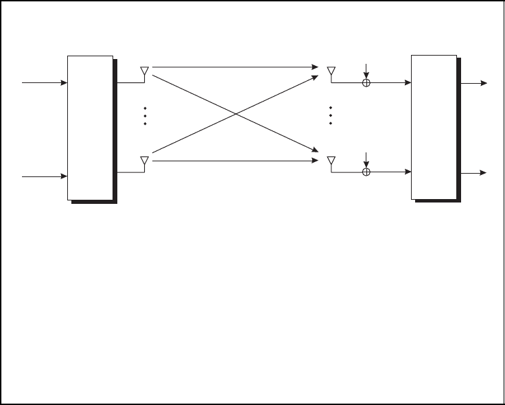
In this chapter, we extend the scenario to multiple-input and multiple-output (MIMO)

systems as depicted in Figure 5.16. The MIMO channel has N

inputs represented by the

signal vector

x[k] =



[k] ··· x

[k]



and N

outputs denoted by

r[k] =



[k] ··· r

[k]



General structure of a frequency-selective MIMO channel

[k]

1,1

[k, κ]

1,N

[k, κ]

[k]

■ Received signal at antenna µ

[k] =



ν=1

−1



κ=0

µ,ν

[k, κ] ·x

[k − κ] +n

[k] (5.26)

■ Entire received signal vector

r[k] =

−1



κ=0

H[k, κ] ·x[k − κ] +n[k] = H[k] · x

[k] + n[k] (5.27)

Figure 5.16: General structure of a frequency-selective MIMO channel

SPACE–TIME CODES 235

Each pair (ν, µ) of transmit and receive antennas is connected by a generally frequency-

selective single-input single-output channel h

µ,ν

[k, κ], the properties of which have already

been described in Chapter 1. At each receive antenna, the N

transmit signals and additive

noise superpose, so that the νth output at time instant k can be expressed as in Equation

(5.26) in Figure 5.16. The parameter L

represents the largest number of taps among all

contributing channels.

A more compact description is obtained by using vector notations. According to

Equation (5.27), the output vector

r[k] =



[k] ··· r

[k]



can be described by the convolution of a sequence of channel matrices

H[k, κ] =







1,1

[k, κ] ··· h

1,N

[k, κ]

[k, κ] ··· h

[k, κ]







with 0 ≤ κ<L

and the input vector x[k] plus the N

dimensional noise vector n[k].

Each row of the channel matrix H[k, κ] contains the coefﬁcients corresponding to a speciﬁc

receive antenna, and each column comprises the coefﬁcients of a speciﬁc transmit antenna,

all for a certain delay κ at time instant k. Arranging all matrices H[k, κ] side by side to an

overall channel matrix

H[k] =



H[k, 0] ··· H[k, L

− 1]



and stacking all input vectors x[k − κ] on top of each other

[k] =



x[k]

··· x[k − L

− 1]



leads to the expression on the right-handside of Equation (5.27) in Figure 5.16.

The general MIMO scenario of Figure 5.16 contains some special cases. For the

frequency-non-selective MIMO case, H[k, κ] = 0

×N

holds for κ>0 and the model

simpliﬁes to

r[k] = H[k] ·x[k] + n[k]

with H[k] = H[k, 0]. Many space–time coding concepts have been originally designed

especially for this ﬂat fading case where the channel does not provide frequency diversity. In

Orthogonal Frequency Division Multiplexing (OFDM) systems with multiple transmit and

receive antennas, the data symbols are spread over different subcarriers each experiencing

a ﬂat fading MIMO channel. Two further cases depicted in Figure 5.17 are obtained if

the transmitter or the receiver deploys only a single antenna. The channel matrix of these

Single-input Multiple-Output (SIMO) systems reduces in this case to a column vector

h[k, κ] =



1,1

[k, κ] ··· h

[k, κ]



By Contrast, the Multiple-Input Single-Output (MISO) system has multiple inputs but only

a single receive antenna and is speciﬁed by the row vector

[k, κ] =



1,1

[k, κ] ··· h

[k, κ]



In order to distinguish between column and row vectors, the latter is underlined. Appro-

priate transmission strategies for MIMO, SIMO and MISO scenarios are discussed in later

sections.