Neubauer A., Freudenberger J., Kuhn V. Coding theory: algorithms, architectures and applications
Подождите немного. Документ загружается.

236 SPACE–TIME CODES
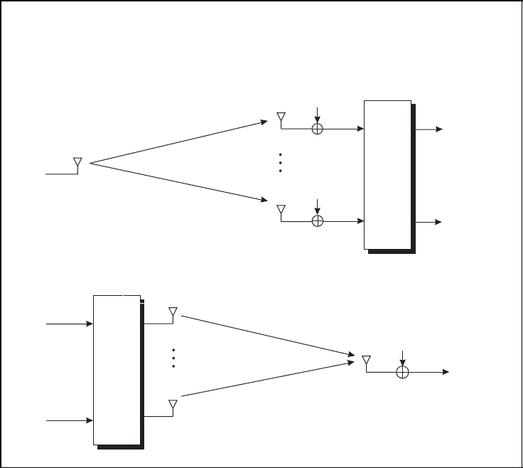
Special MIMO channel
■ Single-Input Multiple-Output (SIMO) channel with N
T
= 1
Rx
x
1
[k]
r
1
[k]
r
N
R
[k]
h
1
[k, κ]
h
N
R
[k, κ]
n
1
[k]
n
N
R
[k]
■ Multiple-Input Single-Output (MISO) channel with N
R
= 1
Tx
x
1
[k]
x
N
T
[k]
r
1
[k]
h
1
[k, κ]
h
N
T
[k, κ]
n
1
[k]
Figure 5.17: Special MIMO channel
Modelling Spatial Channels
In many scientific investigations, the elements in H are assumed to be independent and
identically Rayleigh distributed (i.i.d.). This case assumes a rich scattering environment
without an LoS connection between transmitter and receiver. While this special situation
represents an interesting theoretical point of view and will also be used in this chapter
for benchmarks, real-world scenarios often look different. In many situations, the chan-
nel coefficients in H are highly correlated. This correlation may be caused by a small
distance between neighbouring antenna elements, which is desired for beamforming pur-
poses. For statistically independent coefficients, this distance has to be much larger than
half the wavelength. A second reason for correlations is the existence of only a few
dominant scatterers, leading to preferred directions of departure and arrival and small
angular spreads.

SPACE–TIME CODES 237
Modelling spatial channels
■ General construction of MIMO channel matrix
H[k, κ] =
ν
κ
max
ξ=0
h[k, ξ, θ
R,ν
] · a[k, θ
R,ν
] ·b
T
.
k, θ
T,µ
/
· g[κ −ξ] (5.28)
■ Correlation matrix
HH
= E
vec(H)vec(H)
H
(5.29)
■ Construction of correlated channel matrix from matrix H
w
with i.i.d. ele-
ments
vec(H) =
1/2
HH
· vec(H
w
) (5.30)
■ Simplified model with separated transmitter and receiver correlations
H =
1/2
R
· H
w
·
1/2
T
(5.31)
where
R
(
T
) are assumed to be the same for all transmit (receive)
antennas.
■ Relationship between
HH
,
T
and
R
HH
=
T
T
⊗
R
(5.32)
Figure 5.18: Modelling spatial channels
In practice, only a finite number of propagation paths can be considered. Therefore, the
continuously distributed channel impulse response h(t,τ,θ
R
) will be replaced by a discrete
form h[k, κ,θ
R,ν
].
2
A suitable MIMO channel model represented by a set of matrices H[k, κ] can be
constructed by using Equation (5.28) in Figure 5.18. The vector a[k, θ
R,ν
] denotes the
steering vector at the receiver which depends on the DoA θ
R,ν
as well as the array geometry.
The corresponding counterpart at the transmitter is b
T
[k, θ
T,µ
], where the direction of
departure θ
T,µ
is itself a function of θ
R,ν
and the delay κ. Finally, g[κ] represents the joint
impulse response of transmit and receive filters.
With the assumption that A(·), a[·] and b[·] are sufficiently known, an accurate model of
the space–time channel can be constructed by using correlation matrices as summarised in
2
The time and delay parameters k and κ are generally aligned to the sampling grid on the entire model.
However, we have a finite number of directions of arrival and departure that are not aligned onto a certain grid.
In order to indicate their discrete natures, they are indexed by subscripts ν and µ respectively.

238 SPACE–TIME CODES
Figure 5.18. The exact N
T
N
R
× N
T
N
R
correlation matrix
HH
is given in Equation (5.29),
where the operator vec(A) stacks all columns of a matrix A on top of each other. The
channel matrix H can be constructed from a matrix H
w
of the same size with i.i.d. elements
according to Equation (5.30). To be exact,
HH
should be determined for each delay κ.
However, in most cases
HH
is assumed to be identical for all delays.
A frequently used simplified but less general model is obtained if transmitter and
receiver correlation are separated. In this case, we have a correlation matrix
T
describing
the correlations at the transmitter and a matrix
R
for the correlations at the receiver. The
channel model is now generated by Equation (5.31), as can be verified by
3
E
HH
H
= E
1/2
R
H
w
1/2
T
H/2
T
H
H
w
H H/2
R
=
R
and
E
H
H
H
= E
H/2
T
H
H
w
H/2
R
1/2
R
H
w
1/2
T
=
T
.
A relationship between the separated correlation approach and the optimal one is obtained
with the Kronecker product ⊗, as shown in Equation (5.32).
This simplification matches reality only if the correlations at the transmit side are
identical for all receive antennas, and vice versa. It cannot be applied for pinhole (or
keyhole) channels (Gesbert et al., 2003). They describe scenarios where transmitter and
receiver may be located in rich scattering environments while the rays between them have
to pass a keyhole. Although the spatial fading at transmitter and receiver is mutually
independent, we obtain a degenerated channel of unit rank that can be modelled by
H = h
R
· h
H
T
.
In order to evaluate the properties of a channel, especially its correlations, the Singular
Value Decomposition (SVD) is a suited means. It decomposes H into three matrices: a
unitary N
R
× N
R
matrix U, a quasi-diagonal N
R
× N
T
matrix and a unitary N
T
× N
T
matrix V. While U and V contain the eigenvectors of HH
H
and H
H
H respectively,
=
σ
1
.
.
.
0
r×N
T
−r
σ
r
0
N
R
−r×N
T
−r
contains on its diagonal the singular values σ
i
of H. The number of non-zero singular values
is called the rank of a matrix. For i.i.d. elements in H, all singular values are identical in
the average, and the matrix has full rank as pointed out in Figure 5.19. The higher the
correlations, the more energy concentrates on only a few singular values and the rank of
the matrix decreases. This rank deficiency can also be expressed by the condition number
defined in Equation (5.34) as the ratio of largest to smallest singular value. For unitary
(orthogonal) matrices, it amounts to unity and becomes larger for growing correlations.
The rank of a matrix will be used in subsequent sections to quantify the diversity degree
and the spatial degrees of freedom. The condition number will be exploited in the context
of lattice reduced signal detection techniques.
3
Since H
w
consists of i.i.d. elements, E{H
w
H
H
w
}=I holds.
SPACE–TIME CODES 239
Analysing MIMO channels
■ Singular Value Decomposition (SVD) for flat channel matrix
H = U · · V
H
(5.33)
■ Condition number
κ(H) =
σ
max
σ
min
=H
2
·H
−1
2
≥ 1 (5.34)
–
2
norm of a matrix
H
2
= sup
x=0
Ax
x
(5.35)
– H
2
= σ
max
– H
−1
2
= σ
−1
min
■ Rank of a matrix rank(H) denotes the number of non-zero singular values.
■ Full rank: rank(H) = min{N
T
,N
R
}.
Figure 5.19: Analysing MIMO channels
5.2.3 Channel Estimation
At the end of this section, some principles of MIMO channel estimation are introduced.
Generally, channel knowledge is necessary in order to overcome the disturbing influence of
the channel. This holds for many space–time coding and multilayer transmission schemes,
especially for those discussed in the next sections. However, there exist some exceptions
similar to the concepts of differential and orthogonal modulation schemes for single-input
single-output channels which allow an incoherent reception without Channel State Informa-
tion (CSI). These exceptions are unitary space–time codes (Hochwald and Marzetta, 2000;
Hochwald et al., 2000) and differentially encoded space–time modulation (Hochwald and
Sweldens, 2000; Hughes, 2000; Schober and Lampe, 2002) which do not require any
channel knowledge, either at the transmitter or at the receiver.
While perfect CSI is often assumed for ease of analytical derivations and finding ulti-
mate performance limits, the channel has to be estimated in practice. The required degree
of channel knowledge depends on the kind of transmission scheme. The highest spectral
efficiency is obtained if both transmitter and receiver have channel knowledge. However,
this is the most challenging case. In Time Division Duplex (TDD) systems, reciprocity of
the channel is often assumed, so that the transmitter can use its own estimate obtained in
the uplink to adjust the transmission parameters for the downlink. By contrast, Frequency
Division Duplex (FDD) systems place uplink and downlink in different frequency bands
240 SPACE–TIME CODES
so that reciprocity is not fulfilled. Hence, the transmitter is not able to estimate channel
parameters for the downlink transmission directly. Instead, the receiver transmits its esti-
mates over a feedback channel to the transmitter. In many systems, e.g. UMTS (Holma and
Toskala, 2004), the data rate of the feedback channel is extremely low and error correction
coding is not applied. Hence, the channel state information is roughly quantised, likely to
be corrupted by transmission errors and often outdated in fast-changing environments.
Many schemes do not require channel state information at the transmitter but only at
the receiver. The loss compared with the perfect case is small for medium and high signal-
to-noise ratios and becomes visible only at very low SNRs. Next, we describe the MIMO
channel estimation at the receiver.
Principally, reference-based and blind techniques have to be distinguished. The former
techniques use a sequence of pilot symbols known to the receiver to estimate the channel.
They are inserted into the data stream either as one block at a predefined position in a frame,
e.g. as preamble or mid-amble, or they are distributed at several distinct positions in the frame.
In order to be able to track channel variations, the sampling theorem of Shannon has to be
fulfilled so that the time between successive pilot positions is less than the coherence time of
the channel. By contrast, blind schemes do not need a pilot overhead. However, they generally
have a much higher computational complexity, require rather large block lengths to converge
and need an additional piece of information to overcome the problem of phase ambiguities.
Figure 5.20 gives a brief overview starting with the pilot-assisted channel estimation.
The transmitter sends a sequence of N
P
pilot symbols over each transmit antenna repre-
sented by the (N
T
× N
P
) matrix X
pilot
. Each row of X
pilot
contains one sequence and each
column represents a certain time instant. The received (N
R
× N
P
) pilot matrix is denoted by
R
pilot
and contains in each row a sequence of one receive antenna. Solving the optimisation
problem
ˆ
H
ML
= argmin
˜
H
4
4
4
R
pilot
−
˜
H · X
pilot
4
4
4
2
leads to the maximum likelihood estimate
ˆ
H
ML
as depicted in Equation (5.37). The
Moore–Penrose inverse X
†
pilot
is defined (Golub and van Loan, 1996) by
X
†
pilot
= X
H
pilot
·
X
pilot
X
H
pilot
−1
.
From the last equation we can conclude that the matrix X
pilot
X
H
pilot
has to be invertible, which
is fulfilled if rank(X
pilot
) = N
P
holds, i.e. X
pilot
has to be of full rank and the number of
pilot symbols in X
pilot
has to be at least as large as the number of transmit antennas N
T
.
Depending on the condition number of X
pilot
, the inversion of X
pilot
X
H
pilot
may lead to
large values in X
†
pilot
. Since the noise N is also multiplied with X
†
pilot
, significant noise
amplifications can occur. This drawback can be circumvented by choosing long train-
ing sequences with N
P
>> N
T
, which leads to a large pilot overhead and, consequently,
to a low overall spectral efficiency. Another possibility is to design appropriate training
sequences. If X
pilot
is unitary,
X
pilot
· X
H
pilot
= I
N
T
⇒ X
†
pilot
= X
H
pilot
holds and no noise amplification disturbs the transmission.

SPACE–TIME CODES 241
MIMO channel estimation
■ Pilot-assisted channel estimation:
– Received pilot signal
R
pilot
= H · X
pilot
+ N
pilot
(5.36)
– Pilot-assisted channel estimation
ˆ
H = R
pilot
· X
†
pilot
= H + N
pilot
· X
†
pilot
(5.37)
– Pilot matrix with unitary X
pilot
ˆ
H = R
pilot
· X
H
pilot
= H + N · X
H
pilot
(5.38)
■ Blind channel estimation based on second-order statistics
ˆ
H = E{rr
H
}=E
Hxx
H
H
H
+ nn
H
= σ
2
X
·
R
+ σ
2
N
· I
N
R
(5.39)
Figure 5.20: MIMO channel estimation
A blind channel estimation approach based on second-order statistics is shown in
Equation (5.39). The right-hand side of this equation holds under the assumption of sta-
tistically independent transmit signals E{xx
H
}=σ
2
X
I
N
T
, white noise E{nn
H
}=σ
2
N
I
N
R
and
the validity of the channel model H =
1/2
R
· H
w
·
1/2
T
(cf. Equation (5.31)). It can be
observed that this approach does not deliver phase information. Moreover, the estimate
only depends on the covariance matrix at the receiver, i.e. the receiver cannot estimate cor-
relations at the transmit antenna array with this method. The same holds for the transmitter
in the opposite direction. However, long-term channel characteristics such as directions of
arrival that are incorporated in
R
can be determined by this approach.
5.3 Performance Measures
5.3.1 Channel Capacity
In order to evaluate the quality of a MIMO channel, different performance measures can
be used. The ultimate performance limit is represented by the channel capacity indicating
the maximum data rate that can be transmitted error free. Fixing the desirable data rate by
choosing a specific modulation scheme, the resulting average error probability determines
how reliable the received values are. These quantities have been partly introduced for the
242 SPACE–TIME CODES
scalar case and will now be extended for multiple transmit and receive antennas. We start
our analysis with a short survey for the scalar case.
Channel Capacity of Scalar Channels
Figure 5.21 starts with the model of the scalar AWGN channel in Equation (5.40) and recalls
the well-known results for this simple channel. According to Equation (5.41), the mutual
information between the input x[k] and the output r[k] is obtained from the difference
in the output and noise entropies. For real continuously Gaussian distributed signals, the
differential entropy has the form
I
diff
(X ) = E
− log
2
.
p
X
(x)
/
= 0.5 ·log
2
(2πeσ
2
X
),
while it amounts to
I
diff
(X ) = log
2
(πeσ
2
X
)
for circular symmetric complex signals where real and imaginary parts are statistically
independent and identically distributed. Inserting these results into Equation (5.41) leads to
the famous formulae (5.42b) and (5.42a). It is important to note that the difference between
mutual information and capacity is the maximisation of I(X ;R) with respect to the input
statistics p
X
(x). For the considered AWGN channel, the optimal continuous distribution
of the transmit signal is Gaussian. The differences between real and complex cases can be
AWGN channel capacity
■ Channel output
r[k] = x[k] +n[k] (5.40)
■ Mutual information
I(X ;R) = I
diff
(R) − I
diff
(R | X ) = I
diff
(R) − I
diff
(N ) (5.41)
■ Capacity for complex Gaussian input and noise (equivalent baseband)
C = sup
p
X
(x)
.
I(X ;R)
/
= log
2
1 +
E
s
N
0
(5.42a)
■ Capacity for real Gaussian input (imaginary part not used)
C =
1
2
· log
2
1 + 2
E
s
N
0
(5.42b)
Figure 5.21: AWGN channel capacity

SPACE–TIME CODES 243
explained as follows. On the one hand, we do not use the imaginary part and waste half
of the available dimensions (factor 1/2 in front of the logarithm). On the other hand, the
imaginary part of the noise does not disturb the real x[k], so that the effective SNR is
doubled (factor 2 in front of E
s
/N
0
).
The basic difference between the AWGN channel and a frequency-non-selective fading
channel is its time-varying signal-to-noise ratio γ [k] =|h[k]|
2
E
s
/N
0
which depends on the
instantaneous fading coefficient h[k]. Hence, the instantaneous channel capacity C[k]in
Equation (5.43) is a random variable itself and can be described by its statistical properties.
For fast-fading channels, a coded frame generally spans over many different fading states so
that the decoder exploits diversity by performing a kind of averaging. Therefore, the average
capacity
¯
C among all channel states, termed ergodic capacity and defined in Figure 5.22,
is an appropriate means. In Equation (5.44), the expectation is defined as
E
f(X )
=
-
∞
−∞
f(x)· p
X
(x)dx .
Channel Capacity of Multiple-Input and Multiple-Output Channels
The results in Figure 5.22 can be easily generalised to MIMO channels. The only difference
is the handling of vectors and matrices instead of scalar variables, resulting in multivariate
distributions of random processes. From the known system description
r = H · x + n
of Subsection 5.2.1 we know that r and n are N
R
dimensional vectors, x is N
T
dimen-
sional and H is an N
R
× N
T
matrix. As for the AWGN channel, Gaussian distributed
Scalar fading channel capacities
■ Single-Input Single-Output (SISO) fading channel
r[k] = h[k] · x[k] + n[k]
■ Instantaneous channel capacity
C[k] = log
2
1 +|h[k]|
2
·
E
s
N
0
(5.43)
■ Ergodic channel capacity
¯
C = E{C[k]}=E
%
log
2
1 +|h[k]|
2
·
E
s
N
0
&
(5.44)
Figure 5.22: Scalar fading channel capacities

244 SPACE–TIME CODES
input alphabets achieve capacity and are considered below. The corresponding multivari-
ate distributions for real and complex random processes with n dimensions are shown in
Figure 5.23. The n × n matrix
AA
denotes the covariance matrix of the n-dimensional
process A and is defined as
AA
= E
aa
H
= U
A
·
A
· U
H
A
.
The right-handside of the last equation shows the eigenvalue decomposition (see definition
(B.0.7) in Appendix B) which decomposes the Hermitian matrix
AA
into the diagonal
matrix
A
with the corresponding eigenvalues λ
A,i
,1≤ i ≤ n, and the square unitary
matrix U
A
. The latter contains the eigenvectors of A.
Multivariate distributions and related entropies
■ Joint probability density for a real multivariate Gaussian process
p
A
(a) =
1
√
det(2π
AA
)
· exp
5
−a
T
−1
AA
a/2
6
■ Joint probability density for complex multivariate Gaussian process
p
A
(a) =
1
√
det(π
AA
)
· exp
5
−a
H
−1
AA
a
6
■ Joint entropy of a multivariate process with n dimensions
I
diff
(A) =−E
log
2
[p
A
(a)]
=−
-
A
n
p
A
(a) · log
2
.
p
A
(a)
/
da (5.45)
■ Joint entropy of a multivariate real Gaussian process
I
diff
(A) =
1
2
· log
2
.
det(2πe
AA
)
/
=
1
2
·
n
i=1
log
2
2πeλ
A,i
(5.46a)
■ Joint entropy of a multivariate complex Gaussian process
I
diff
(A) = log
2
.
det(πe
AA
)
/
=
n
i=1
log
2
πeλ
A,i
(5.46b)
Figure 5.23: Multivariate distributions and related entropies
SPACE–TIME CODES 245
Following Figure 5.23, we recognize from Equation (5.45) that the differential entropy
I
diff
(X ) is defined in exactly the same way as for scalar processes except for the expec-
tation (integration) over an N
T
-dimensional space. Solving the integrals by inserting the
multivariate distributions for real and complex Gaussian processes, we obtain the differ-
ential entropies in Equations (5.46a) and (5.46b). They both depend on the covariance
matrix
AA
. Using its eigenvalue decomposition and the fact that the determinant of a
matrix equals the product of its eigenvalues, we obtain the right-hand-side expressions
of Equations (5.46a) and (5.46b). If the elements of A are statistically independent and
identically distributed (i.i.d.), all with variance λ
A,i
= σ
2
A
, the differential entropy becomes
I
diff
(A) = log
2
7
n
i=1
(πeλ
A,i
)
8
=
n
i=1
log
2
πeλ
A,i
=
i.i.d.
n · log
2
πeσ
2
A
for the complex case. An equivalent expression is obtained for real processes.
Using the results of Figure 5.23, we can now derive the capacity of a MIMO channel. A
look at Equation (5.47) in Figure 5.24 illustrates that the instantaneous mutual information
Mutual Information of MIMO systems
■ Mutual information of a MIMO channel
I(X ;R | H) = I
diff
(R | H) − I
diff
(N ) = log
2
det(
RR
)
det(
NN
)
(5.47)
■ Inserting SVD H = U
H
H
V
H
H
and
NN
= σ
2
N
I
N
R
I(X ;R | H) = log
2
det
I
N
R
+
1
σ
2
N
H
V
H
H
XX
V
H
H
H
(5.48)
■ Perfect channel knowledge only at receiver
I(X ;R | H) = log
2
det
I
N
R
+
σ
2
X
σ
2
N
H
H
H
=
N
T
i=1
log
2
1 + σ
2
H,i
·
σ
2
X
σ
2
N
(5.49)
■ Perfect channel knowledge at transmitter and receiver
I(X ;R | H) = log
2
det
I
N
R
+
1
σ
2
N
H
X
H
H
=
N
T
i=1
log
2
1 + σ
2
H,i
·
σ
2
X ,i
σ
2
N
(5.50)
Figure 5.24: Mutual Information of MIMO systems