Patrick F. Dunn, Measurement, Data Analysis, and Sensor Fundamentals for Engineering and Science, 2nd Edition

Подождите немного. Документ загружается.

146 Measurement and Data Analysis for Engineering and Science

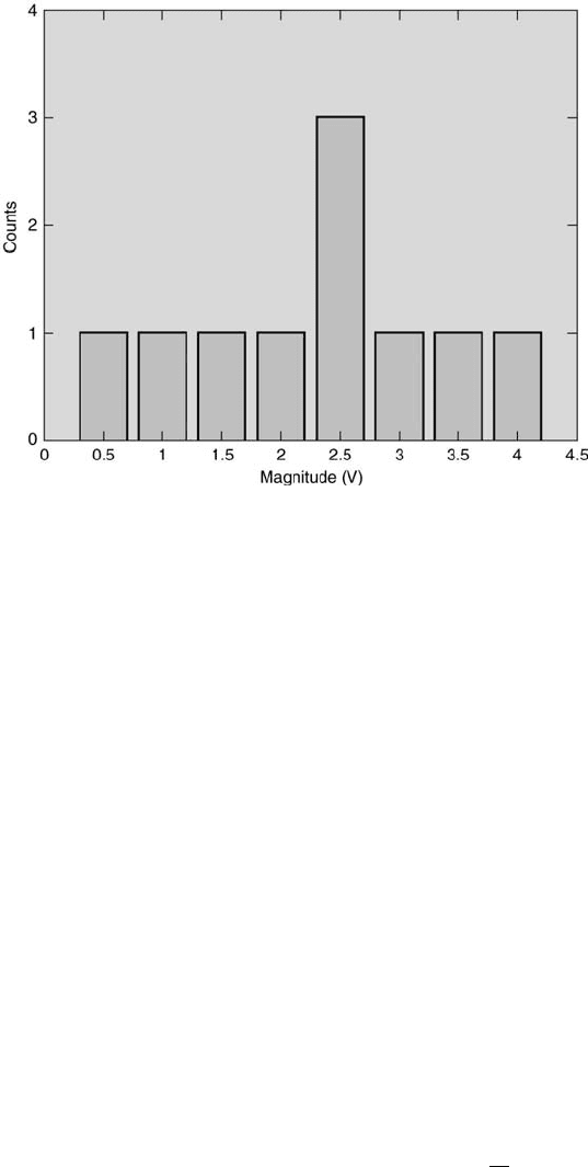
FIGURE 5.3

The histogram of a digital signal representation.

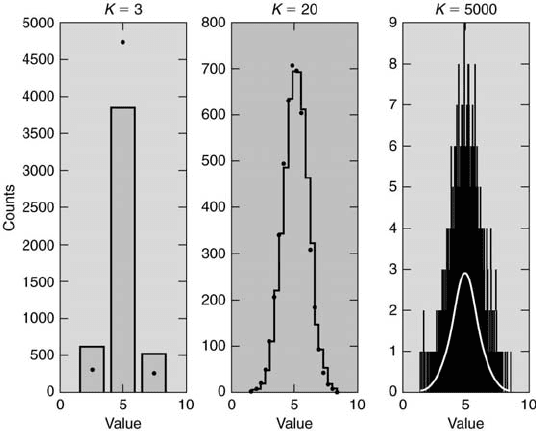
representative histogram. An example of how the choice of the number of

intervals aﬀects the histogram’s ﬁdelity is presented in Figure 5.4. In that

ﬁgure, the theoretical values of the population are represented by black dots

in the left and center histograms and by a white curve in the right histogram.

The data used for the histogram consisted of 5000 values drawn randomly

from a normally distributed population (this type of distribution is discussed

in Chapter 6). In the left histogram, too few intervals are chosen and the

population is over-estimated in the left and right bins and under-estimated

in the center bin. In the right histogram, too many intervals are chosen and

the population is consistently over-estimated in almost all bins. In the middle

histogram, the optimum number of class intervals is chosen and excellent

agreement between the observed and expected values is achieved.

For equal-probability interval histograms, the intervals have diﬀerent

widths. The widths typically are determined such that the probability of

an interval equals 1/K, where K denotes the number of intervals. Bendat

and Piersol [17] present a formula for K that was developed originally for

continuous distributions by Mann and Wald [11] and modiﬁed by Williams

[12]. It is valid strictly for N ≥ 450 at the 95 % conﬁdence level, although

Mann and Wald [11] state that it is probably valid for N ≥ 200 or even

lower N. The exact expression given by Mann and Wald is K = 2[2(N −

]

0.2

, where c = 1.645 for 95 % conﬁdence. Various spreadsheets as well

as Montgomery and Runger [6] suggest the formula K =

√

N, which agrees

Probability 147

FIGURE 5.4

Histograms with diﬀerent numbers of intervals for the same data.

within 10 % with the modiﬁed Mann and Wald formula up to approximately

N = 1000.

For equal-width interval histograms, the interval width is constant and

equal to the range of values (maximum minus minimum values) divided by

the number of intervals. Sturgis’ formula [10] determines K from the number

of binomial coeﬃcients needed to have a sum equal to N and can be used for

values of N as low as approximately 30. Based upon this formula, various

authors, such as Rosenkrantz [5], suggest using values of K between 5 and 20

(this would cover between approximately N = 2

= 32 to N = 2

' 10

Scott’s formula for K ([13] and [14]), valid for N ≥ 25, was developed to

minimize the integrated mean square error that yields the best ﬁt between

Gaussian data and its parent distribution. The exact expression is ∆x =

3.49σN

−1/3

, where ∆x is the interval width and σ the standard deviation.

Using this expression and assuming a range of values based upon a certain

percent coverage, an expression for K can be derived.

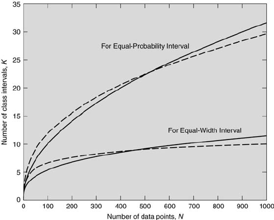
The formulas for K for both types of histograms are presented in Ta-

ble 5.1 and displayed in Figure 5.5. The number of intervals for equal-

probability interval histograms at a given value of N is approximately two

to three times greater than the corresponding number for equal-width inter-

val histograms. More intervals are required for the former case because the

center intervals must be narrow and numerous to maintain the same proba-

bility as those intervals on the tails of the distribution. Also, because of the

148 Measurement and Data Analysis for Engineering and Science

FIGURE 5.5

K = f(N) formulas for equal-width and equal-probability histograms. Equal-

probability interval symbols: modiﬁed Mann and Wald formula (dash) and

square-root formula (solid). Equal-width interval symbols: Sturgis formula

(dash) and Scott formula (solid).

low probabilities of occurrence at the tails of the distribution, some inter-

vals for equal-width histograms may need to be combined to achieve greater

than ﬁve occurrences in an interval. This condition (see [14]) is necessary

for proper comparison between theoretical and experimental distributions.

However, for small samples it may not be possible to meet this condition.

Another very important condition that must be followed is that ∆x ≥ u

where u

is the uncertainty of the measurement of x. That is, the interval

width should never be smaller than the uncertainty of the measurand.

To construct equal-width histograms, these steps must be followed:

1. Identify the minimum and maximum values of the measurand x, x

min

and x

max

, thereby ﬁnding its range, x

range

= x

max

− x

min

2. Determine the number of class intervals, K, using the appropriate for-

mula for equal-width histograms. Preferably, this should be Scott’s for-

mula.

3. Calculate the width of each interval, where ∆x = x

range

/K.

Probability 149

Interval Type

Formula

Reference

Equal-probability

K = 1.87(N −1)

0.40

[11], [12], [17]

Equal-probability

K =

√

[6], [15]

Equal-width

K = 3.322 log

[10]

Equal-width

K = 1.15N

1/3

[13], [14]

TABLE 5.1

Formulas for the number of histogram intervals with 95 % conﬁdence.

4. Count the number of occurrences, n

(j = 1 to K), in each ∆x interval.

Check that the sum of all the n

’s equals N, the total number of data

points.

5. Check that the conditions for n

> 5 (if possible) and ∆x ≥ u

(deﬁ-

nitely) are met.

6. Plot n

vs xm

, where xm

is discretized as the mid-point value of each

interval.

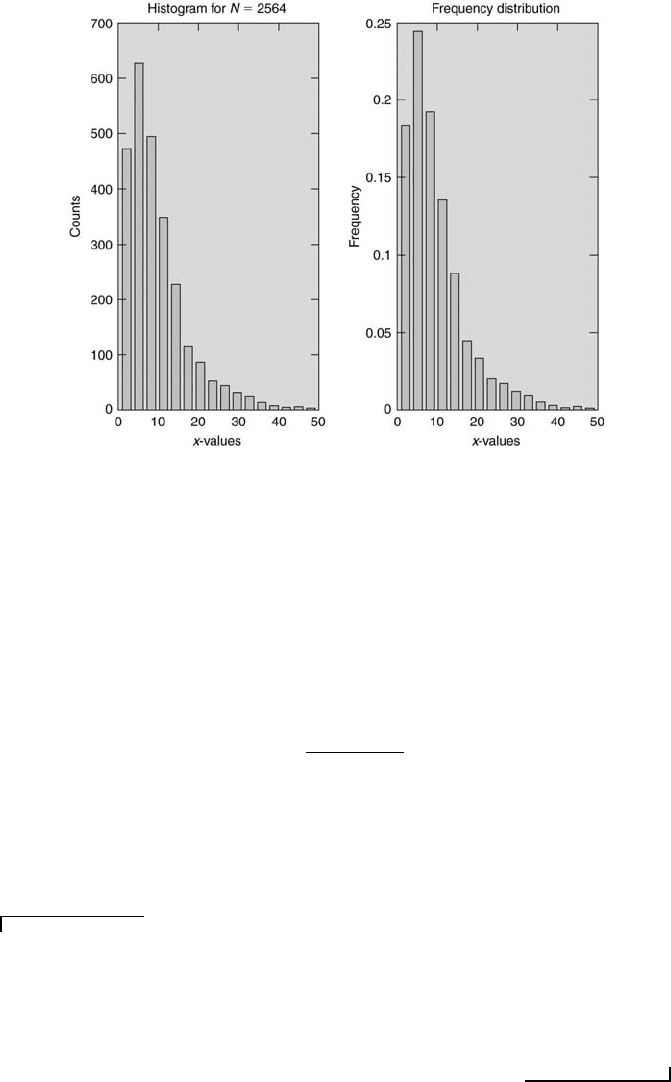
Instead of examining the distribution of the number of occurrences of

various magnitudes of a signal, the frequency of occurrences can be deter-

mined and plotted. The plot of n

/N = f

versus xm

is known as the

frequency distribution (sometimes called the relative frequency distri-

bution). The area bounded laterally by any two x values in a frequency

distribution equals the frequency of occurrence of that range of x values or

the probability that x will assume values in that range. Also, the sum of all

the f

’s equals 1. The frequency distribution often is preferred over the his-

togram because it corresponds to the probabilities of occurrence. Further, as

the sample size becomes large, the sample’s frequency distribution becomes

similar to the distribution of the population’s probabilities, which is called

the probability density function.

The distribution of all of the values of the inﬁnitely large population

is given by its probability density function, p(x). This will be deﬁned in

the next section. Typically p(x) is normalized such that the integral of p(x)

over all x equals unity. This eﬀectively sets the sum of the probabilities of

all the values between −∞ and +∞ to be unity or 100 %. Similar to the

frequency distribution, the area under the portion of the probability density

function over a given measurand range equals the percent probability that

the measurands will have values in that range.

To properly compare a frequency distribution with an assumed proba-

bility density function on the same graph, the frequency distribution ﬁrst

must be converted into a frequency density distribution. The frequency

density is denoted by f

∗

, where f

∗

= f

/∆x. This is because the probability

density function is related to the frequency distribution by the expression

150 Measurement and Data Analysis for Engineering and Science

FIGURE 5.6

Sample histogram and frequency distributions of the same data.

p(x) = lim

N→∞,∆x→0

j=1

/∆x = lim

N→∞,∆x→0

j=1

∗

. (5.1)

The N required for this comparative limit to be attained within a certain

conﬁdence can be determined using the law of large numbers [5], which is

N ≥

4

(1 − P

)

. (5.2)

This law, derived by Jacob Bernoulli (1654-1703), considered the father of

the quantiﬁcation of uncertainty, was published posthumously in 1713 [1].

The law determines the N required to have a probability of at least P

that

∗

(x) diﬀers from p(x) by less than .

Example Problem 5.1

Statement: One would like to determine whether or not a coin used in a coin toss

is fair. How many tosses would have to be made to assess this?

Solution: Assume one wants to be at least 68 % conﬁdent (P

= 0.68) that the

coin’s fairness is assessed to within 5 % ( = 0.05). Then, according to Equation 5.2,

the coin must be tossed at least 310 times (N ≥ 310).

Probability 151

Often the frequency distribution of a ﬁnite sample is used to identify the

probability density function of its population. The probability density func-

tion’s shape tells much about the physical process governing the population.

Once the probability density function is identiﬁed, much more information

about the process can be obtained.

5.5 Probability Density Function

Consider the time history record of a random variable, x(t). Its probability

density function, p(x), reveals how the values of x(t) are distributed over

the entire range of x(t) values. The probability that x(t) will be between x

∗

and x

∗

+ ∆x is given by

p(x) = lim

∆x→0

P r[x

∗

< x(t) ≤ x

∗

+ ∆x]

∆x

. (5.3)

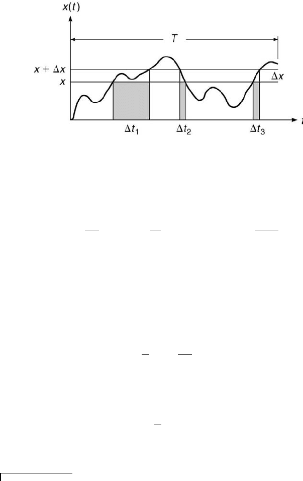
The probability that x(t) is in the range x to x + ∆x over a total time

period T also can be determined. Assume that T is large enough such that

the statistical properties are truly representative of that time history. Fur-

ther assume that a single time history is suﬃcient to fully characterize the

underlying process. These assumptions are discussed further in Chapter 9.

For the time history depicted in Figure 5.7, the total amount of time during

the time period T that the signal is between x and x + ∆x is given by T

where

j=1

∆t

(5.4)

for m occurrences. In other words,

P r[x < x(t) ≤ x + ∆x] = lim

T →∞





= lim

T →∞

j=1

∆t

. (5.5)

This implies that

p(x) = lim

∆x→0

∆x





lim

T →∞

j=1

∆t





= lim

∆x→0,T →∞



∆x



. (5.6)

Likewise, x could be the number of occurrences of a variable with a ∆x

interval, n

, where the total number of occurrences is N . Here N is like T

and n

is like T

, so

152 Measurement and Data Analysis for Engineering and Science

FIGURE 5.7

A time history record.

p(x) = lim

∆x→0

∆x





lim

N→∞

j=1





= lim

∆x→0,N→∞

j=1



∆x



. (5.7)

Equations 5.6 and 5.7 show that the limit of the frequency density distribu-

tion is the probability density function.

The probability density function of a signal that repeats itself in time

can be found by applying the aforementioned concepts. To determine the

probability density function of this type of signal, the signal only needs to

be examined over one period T . Equation 5.6 then becomes

p(x) =

lim

∆x→0

∆x

j=1

∆t

. (5.8)

Now as ∆x → 0, ∆t

→ ∆x · |dt/dx|

. Thus, in the limit as ∆x → 0,

Equation 5.8 becomes

p(x) =

j=1

|dt/dx|

, (5.9)

noting that m is the number of times the signal is between x and x + ∆x.

Example Problem 5.2

Statement: Determine the probability density function of the periodic signal x(t) =

sin(ωt) with ω = 2π/T .

Solution: Diﬀerentiation of the signal with respect to time yields

dx = x

ω cos(ωt)dt or dt = dx/[x

ω cos(ωt)]. (5.10)

Probability 153

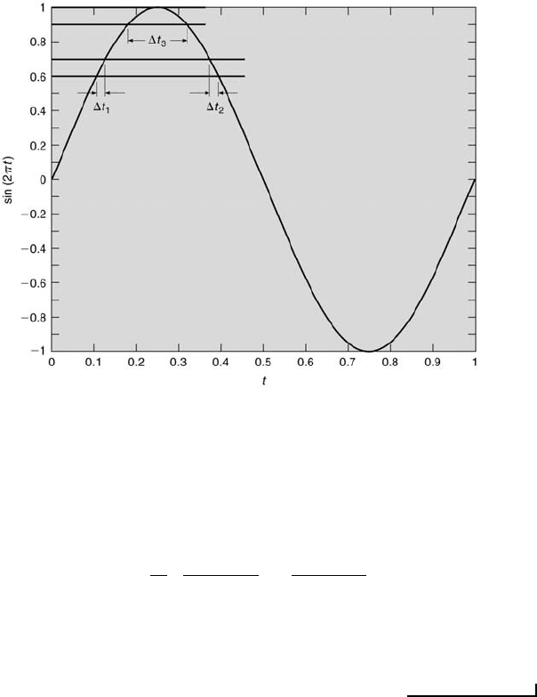
FIGURE 5.8

Constructing p(x) from the time history record.

Now, the number of times that this particular signal resides during one period in the

x to x + ∆x interval is 2. Thus, for this signal, using Equations 5.9 and 5.10, the

probability density function becomes

p(x) =

2π

ω cos(ωt)

| = |

πx

cos(ωt)

|. (5.11)

The probability density functions of other deterministic, continuous functions of

time can be found using the same approach.

The probability density function also can be determined graphically by

analyzing the time history of a signal in the following manner:

1. Given x(t) and the sample period, T , choose an amplitude resolution

∆x.

2. Determine T

, then T

/(T ∆x), noting also the mid-point value of x for

each ∆x interval.

3. Construct the probability density function by plotting T

/(T

∆x) for

each interval on the ordinate (y-axis) versus the mid-point value of x for

that interval on the abscissa (x-axis).

154 Measurement and Data Analysis for Engineering and Science

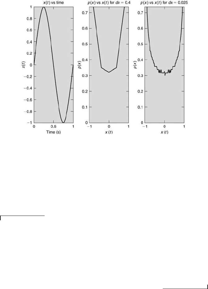
FIGURE 5.9

Approximations of p(x) from x(t) = sin(2πt).

Note that the same procedure can be applied to examining the time history

of a signal that does not repeat itself in time. By graphically determining the

probability density function of a known periodic signal, it is easy to observe

the eﬀect of the amplitude resolution ∆x on the resulting probability density

function in relation to the exact probability density function.

Example Problem 5.3

Statement: Consider the signal x(t) = x

sin(2πt/T ). For simplicity, let x

= 1

and T = 1, so x = sin(2πt). Describe how the probability density function could be

determined graphically.

Solution: First choose ∆x = 0.10. As illustrated in Figure 5.8, for the interval

0.60 < sin(2πt) ≤ 0.70, T

= 0.020 + 0.020 = 0.040, which yields T

/(T

∆x) = 0.40

for the mid-point value of x = 0.65. Likewise, for the interval 0.90 < sin(2πt) ≤ 1.00,

= 0.14, which yields T

/(T ∆x) = 1.40 for the mid-point value of x = 0.95. Using

this information gathered for all ∆x intervals, an estimate of the probability density

function can be made by plotting T

/(T/∆x) versus x.

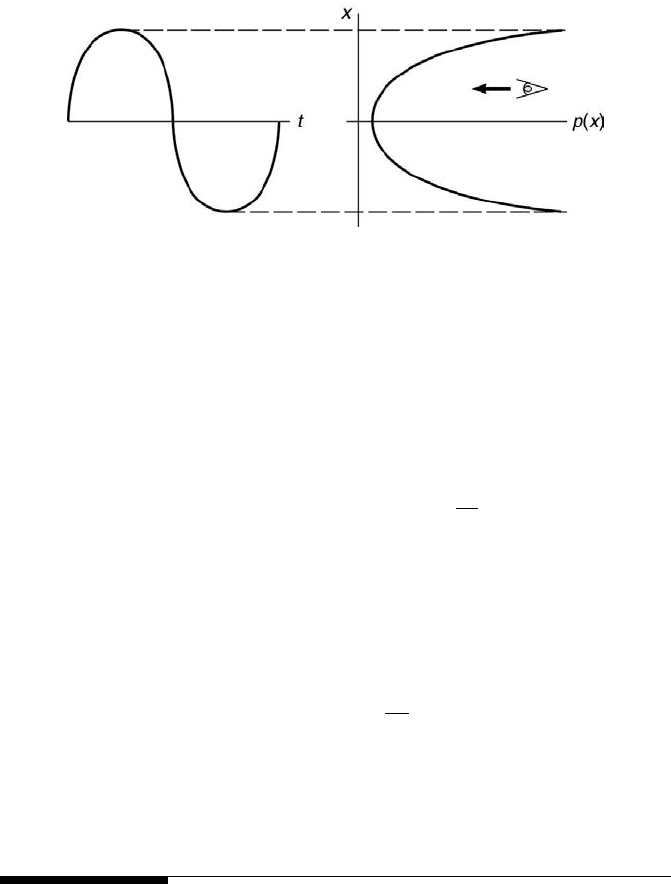
One simple way of interpreting the underlying probability density func-

tion of a signal is to consider it as the projection of the density of the signal’s

amplitudes, as illustrated below in Figure 5.10 for the signal x = sin(2πt).

The more frequently occurring values appear more dense as viewed along

the horizontal axis.

Probability 155

FIGURE 5.10

Projection of signal’s amplitude densities.

In some situations, particularly when examining the time history of a

random signal, the aforementioned procedure of measuring the time spent

at each ∆x interval to determine p(x) becomes quite laborious. Recall that

if p(x)dx is known, the probability of occurrence of x for any range of x is

given by

p(x)dx = lim

∆x→0

p(x)∆x = lim

T →∞





. (5.12)

Recognizing this, an alternative approach can be used to determine the

quantity p(x)dx by choosing a very small ∆x, such as the thickness of a

pencil line. If a horizontal line is moved along the amplitude axis at constant-

amplitude increments and the number of times that the line crosses the

signal is determined for each amplitude increment, C

, then

p(x)dx = lim

C→∞





, (5.13)

where C is a very large number. Note that p(x)dx was determined by this

approach, not p(x), as was done previously.

5.6 Various Probability Density Functions

The concept of the probability density function was introduced in Chapter

5. There are many speciﬁc probability density functions. Each represents a

diﬀerent population that is characteristic of some physical process. In the

following, a few of the more common ones will be examined.

Some of the probability density functions are for discrete processes (those

having only discrete outcomes), such as the binomial probability density