Schneider P., Eberly D.H. Geometric Tools for Computer Graphics
Подождите немного. Документ загружается.

154 Chapter 4 Matrices, Vector Algebra, and Transformations
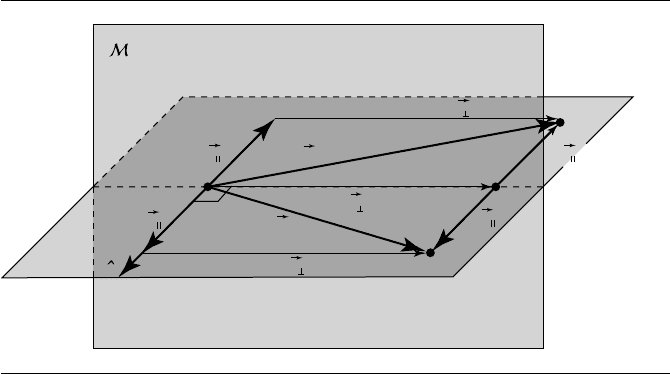
Q
P
T(P)
v
v
v
v
T(v ) T(v )
T(v )
T(v)
v
n
Figure 4.22 Mirror image in 3D.
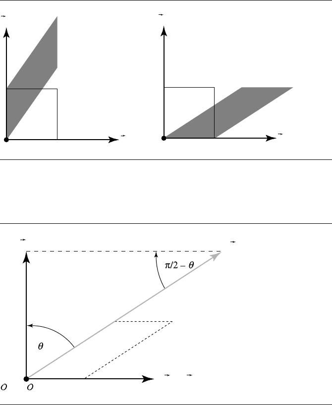
Simple Shearing
Shearing, in general, may be done along any line (in 2D) or orthogonally to any plane
(in 3D), but as with the other transforms, we’ll discuss the simple cases first. The sim-
ple shears are done along the basis vectors and through the origin. Shears, as can be
seen in Figure 4.23, transform rectangles into parallelograms; these parallelograms,
however, must have the same area as the original rectangle. As any parallelogram has
its area as base × height, it should be clear why the simple shears preserve either the
base or height of an axis-aligned rectangle.
There are numerous options for specifying a simple shear. The one we’ll use here
specifies the axis along which the shearing takes place and the shearing angle; other
books, such as M
¨
oller and Haines (1999), specify a shearing scale rather than an
angle.
Again we’ll construct a transformation matrix by considering in turn what the
transformation must do to the basis vectors and origin of our frame. We’ll show a
shear along the x-axis (the right-hand image in Figure 4.23); we’ll refer to this as T
xy,θ
(the reason for the subscript being xy rather than just x will be more clear when we
cover 3D shearing).
First, let’s consider the image of v
1
—the x-axis, under T
xy,θ
. As can be seen in
Figure 4.24, the x-axis remains unchanged:
T
xy,θ
(v
1
) =v
1
=
[
100
]
4.7 Vector Geometry of Affine Transformations 155
v
1
v
2
v
1
v
2
Figure 4.23 Shearing in 2D.
T(v
1
) = v
1
v
2
T(v
2
)
= T( )
Figure 4.24 T
xy,θ
.
The image of v
2
—the y-axis, under T
xy,θ
—can be computed in the following
fashion: if we consider the right triangle formed by the origin O and the points
O +v
2
and O + T(v
2
), the angle whose vertex is at O is θ . If we recall that v
2
=1
(because we’re assuming standard Euclidean basis), we can use simple trigonometry
to deduce the image of v
2
under T
xy,θ
:
156 Chapter 4 Matrices, Vector Algebra, and Transformations
T
xy,θ
(v
2
) =
[
tan θ 10
]
Finally, T clearly has no effect on the origin O,sowehave
T(O) = O
=
[
001
]
and thus our transformation matrix is
T
xy,θ
=
T(v
1
)
T(v
2
)
T(O)
=
100
tan θ 10
001
A similar approach for T
yx,θ
(a shear in the y-direction) yields
T
yx,θ
=
1 tan θ 0
010
001
In three dimensions, there are six different shears. If we let
H
ηγ
= tan θ
ηγ
where η specifies which coordinate is being changed by the shearing matrix and γ
specifies which coordinate does the shearing, then the following schematic can be
constructed that shows the placement of the shearing factor to get the desired shear
direction:
1 H
yx
H
zx
0
H
xy
1 H
zy
0
H
xz
H
yz
10
0001
Only one of these H factors should be nonzero. The composition of two or more
shears must be implemented by forming each shear matrix and multiplying the ma-
trices together.
4.7 Vector Geometry of Affine Transformations 157
v
Q
P
P'
P"
ˆv
ˆn
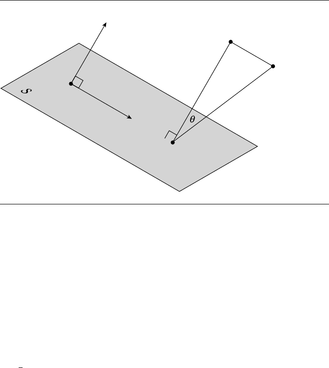
Figure 4.25 General shear specification.
General Shearing
A more general shear is defined by a shearing plane S, unit vector ˆv in S, and
shear angle θ . The plane S is defined by a point Q on the plane and a normal ˆn.
The shear transform moves a family of parallel planes in space so that the planes
remain parallel; one plane (the one defining it) is unmoved. Goldman (1991) gives
the construction of a shearing transform matrix (see Figure 4.25): for any point P ,let
P
be its orthogonal projection on S; then, construct point P
=P + t ˆv with t such
that
P
P
P =θ. If we apply a shear transform to P ,wegetP
. The transformation
is
T
Q,ˆn,v,θ
=
I +tan θ(ˆn ⊗ˆv)
0
T
−(Q ·ˆn) ˆv 1
Goldman notes that the determinant of this matrix is 1, and thus the shear transfor-
mation preserves volumes (note that −π/2 <θ<π/2).
The general 3D shear matrix can be constructed along different lines, and perhaps
more simply. The vectors ˆv and ˆn, along with the point Q, define an affine frame (the
third basis vector is ˆv ׈n). If we have a point P =Q +y
1
ˆn +y
2
ˆv + y
3
( ˆn ׈v), then
the shearing operation would map that point to
158 Chapter 4 Matrices, Vector Algebra, and Transformations
T(P)= T (Q) + y
1
T(ˆn) + y
2
T(ˆv) + y
3
T(ˆn ׈v)
= Q + y
1
( ˆn + tan θ ˆv) + y
2
ˆv + y
3
( ˆn ׈v)
= Q + y
1
ˆn + (y
2
+ y
1
tan θ)ˆv + y
3
( ˆn ׈v)
The matrix relative to the affine frame is
1 tan θ 00
0100
0010
Q
x
Q
y
Q
z
1
whose upper-left 3 ×3blockH the reader should recognize as the 2D y-shear matrix
T
yx,θ
from the previous section (the basis vector v is acting as the y-axis for that
frame).
In terms of the standard Euclidean basis, if we have a rotation matrix
R =
ˆn
ˆv
ˆn ׈v
and
y =
[
y
1
y
2
y
3
]
then
P = Q +yR
and
T(P)= Q +yHR
= Q + (P − Q)R
T
HR
The matrix T for T is
T
ˆn,ˆv,Q,θ
=
R
T
HR
0
T
Q(I
3
− R
T
HR) 1
4.8 Projections
Projections are a class of transformations that all share the characteristic that they
transform points from an n-dimensional frame (coordinate system) to a frame with
4.8 Projections 159
less than n dimensions (generally, n − 1). The most significant use of projection
in computer graphics is in the rendering pipeline of graphics display systems and
libraries, where three-dimensional objects are projected onto a plane before being
rasterized and displayed on a terminal screen.
The class of projective transformations contains two subclasses that are of par-
ticular interest in computer graphics: parallel and perspective. A projection can be
defined as the result of taking the intersection of a line connected to each point on a
geometric object with a plane. In parallel projection, all of these projectors are paral-
lel, while in perspective projection, the projectors meet at a common point, referred
to as the center of projection. As pointed out in Foley et al. (1996, Section 6.1), you
can justifiably consider the center of projection in a parallel projection to be a point
at infinity.
In the following sections, we’ll show how orthographic and perspective projection
transformation matrices can be constructed using only vector algebra techniques.
For a thorough treatment of the various subclasses of parallel projections, and the
construction of parallel and perspective projection transformation matrices for the
purposes of creating viewing transformations, see Foley et al. (1996, Chapter 6).
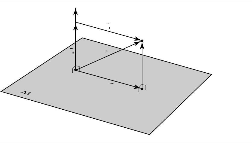
4.8.1 Orthographic
Orthographic projection (also called orthogonal) is the simplest type of projection
we’ll discuss: it consists of merely projecting points and vectors in a perpendicular
fashion onto a plane, as shown in Figure 4.26. As in the case of the mirror transform,
we define the plane M byapointQ on the plane and (unit) normal vector ˆu.
Orthographic projection of a vector v is simply the usual sort of projection we’ve
been using all along: we project v onto ˆu to get the parallel and perpendicular com-
ponents, and note that since v
⊥
is position independent, the relative location of Q is
not considered. Thus, we have
T(v) =v
⊥
=v −(v ·ˆu) ˆu
(4.33)
The transformation of a point P is similarly trivial:
T(P)= Q + T(v)
= Q + T(P − Q)
= P −((P − Q) ·ˆu) ˆu
(4.34)
The matrix representation of this is accomplished by factoring out v from Equa-
tion 4.33 to give the upper left-hand n × n submatrix:
T
ˆu
=
I −( ˆu ⊗ˆu)
160 Chapter 4 Matrices, Vector Algebra, and Transformations
Q
P
v
T(P)
T(v)
v
v
û
Figure 4.26 Orthographic (orthogonal) projection.
The bottom row is computed as usual by factoring out the above and the point P
from Equation 4.34:
T
ˆu,Q
=
T
ˆu
0
T
(Q ·ˆu) ˆu 1
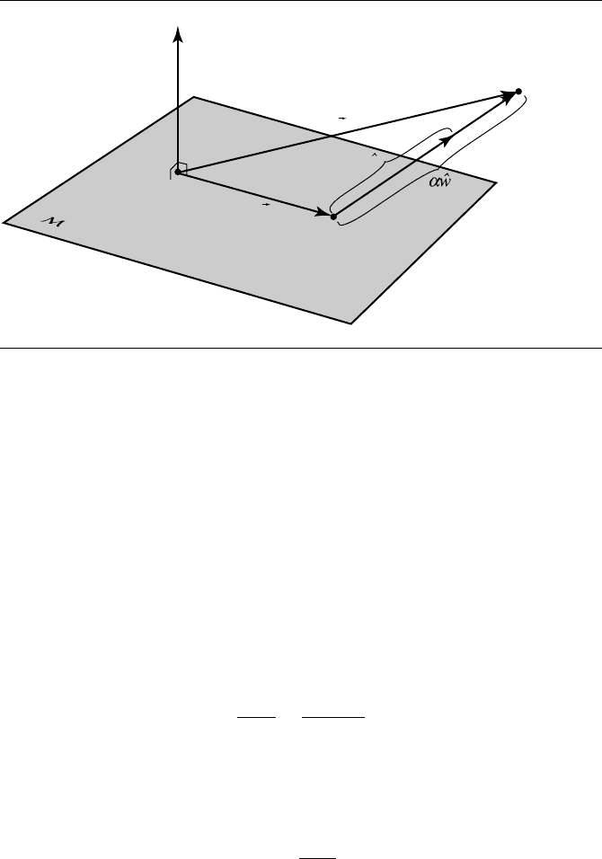
4.8.2 Oblique
Oblique (or parallel) projection is simply a generalization of orthographic
projection—the projection is parallel, but the plane need not be perpendicular to
the projection “rays.” Again, the projection plane M is defined by a point Q on it
and a normal vector ˆu, but since ˆu no longer also defines the direction of projection,
we need to specify another (unit) vector ˆw as the projection direction, as shown in
Figure 4.27.
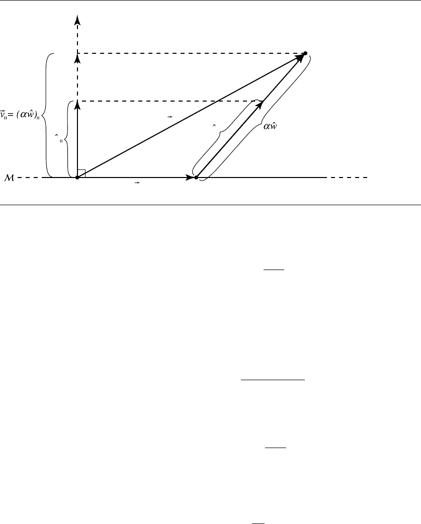
An edge-on diagram of this (Figure 4.28) will help us explain how to determine
the transformation of vectors. We can start out by observing that
v = T(v) + α ˆw
4.8 Projections 161
Q
P
v
T(P)
T(v)
w
û
Figure 4.27
Oblique projection.
which we can rearrange as
T(v) =v −α ˆw (4.35)
Obviously, what we need to compute is α, but this is relatively straightforward, if
we realize that
v
=(α ˆw)
We can exploit this as follows:
v
ˆw
=
(α ˆw)
ˆw
= α
which we can rewrite using the definition of the dot product:
α =
v ·ˆu
ˆw ·ˆu
(4.36)
We then can substitute Equation 4.36 into Equation 4.35 to get the transformation
for vectors:
162 Chapter 4 Matrices, Vector Algebra, and Transformations
Q
P
v
T(P)
T(v )
w
û
w
Figure 4.28 Edge-on view of oblique projection.
T(v) =v −
v ·ˆu
ˆw ·ˆu
ˆw (4.37)
We can then, as usual, employ the definition of point and vector addition and sub-
traction to obtain the formula for transforming a point:
P = Q + T(v)
= Q + T(P − Q)
= P −
((P − Q) ·ˆu) ˆw
ˆw ·ˆu
(4.38)
To convert this to matrix representation, we apply the usual technique of extract-
ing v from Equation 4.37 to compute the upper left-hand n × n submatrix:
T
ˆu, ˆw
=
I −
( ˆu⊗ˆw)
ˆw·ˆu
To compute the bottom row of the transformation matrix, we extract that and the P
from Equation 4.38, and the complete matrix looks like this:
T
ˆu,Q, ˆw
=
T
ˆu, ˆw
0
T
Q·ˆu
ˆw·ˆu
ˆw 1
4.8 Projections 163
Q
S
P
T(P)
P
2
T(P
2
)
T(P
3
)
P
3
û
Figure 4.29 Perspective projection.
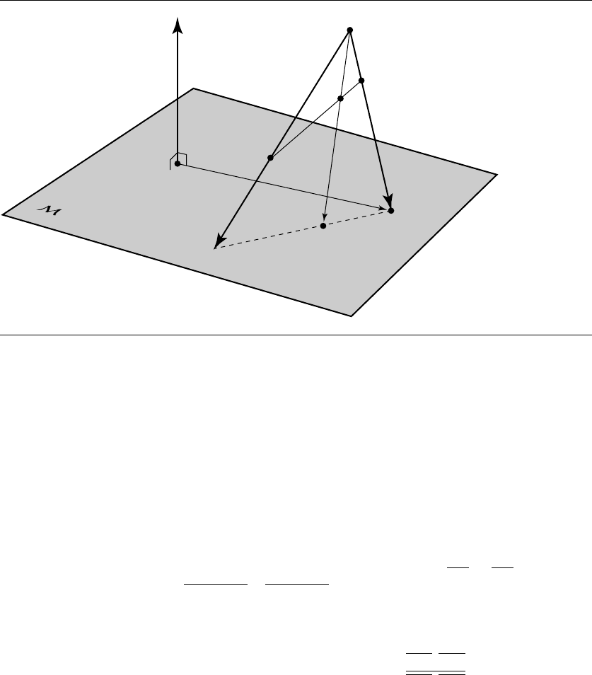
4.8.3 Perspective
Perspective projection is not an affine transformation; it does not map parallel lines
to parallel lines, for instance. Unlike the orthographic and parallel projections, the
projection vectors are not uniform for all points and vectors; rather, there is a pro-
jection point or perspective point, and the line of projection is defined by the vector
between each point and the perspective point, as shown in Figure 4.29.
Perspective projection does, however, preserve something called cross-ratios.Re-
call that affine maps preserve ratios: given three collinear points P , R, and Q, the
ratio of the distance between P and R (which we notate as
PR)to
RQ is the same as
the ratio of
T(P)T(R)to T(R)T(Q)(see Figure 3.36).
The cross-ratio is defined as follows: given four collinear points P , R
1
, R
2
, and Q,
the cross-ratio is
CrossRatio(P , R
1
, R
2
, Q) =
PR
1
/R
1
Q
PR
2
/R
2
Q
as shown on the left side of Figure 4.30. Preservation of cross-ratio means that the
following holds: