Schneider P., Eberly D.H. Geometric Tools for Computer Graphics
Подождите немного. Документ загружается.

244 Chapter 7 Intersection in 2D
// lines are the same
return 2;
}
The pseudocode for the intersection of two line segments is presented below. The
return value of the function is 0 if there is no intersection, 1 if there is a unique
intersection, and 2 if the two segments overlap and the intersection set is a segment
itself. The return value is the number of valid entries in the array
I[2] that is passed to
the function. Relative error tests are used in the same way as they were in the previous
function.
int FindIntersection(Point P0, Point D0, Point P1, Point D1, Point2 I[2])
{
// segments P0+s*D0forsin[0,1],P1+t*D1fortin[0,1]
PointE=P1-P0;
float kross = D0.x * D1.y - D0.y * D1.x;
float sqrKross = kross * kross;
float sqrLen0 = D0.x * D0.x + D0.y * D0.y;
float sqrLen1 = D1.x * D1.x + D1.y * D1.y;
if (sqrKross > sqrEpsilon * sqrLen0 * sqrLen1) {
// lines of the segments are not parallel
float s = (E.x * D1.y - E.y * D1.x) / kross;
if(s<0ors>1){
// intersection of lines is not a point on segment P0+s*D0
return 0;
}
float t = (E.x * D0.y - E.y * D0.x) / kross;
if(t<0ort>1){
// intersection of lines is not a point on segment P1+t*D1
return 0;
}
// intersection of lines is a point on each segment
I[0]=P0+s*D0;
return 1;
}
// lines of the segments are parallel
float sqrLenE = E.x * E.x + E.y * E.y;
kross = E.x * D0.y - E.y * D0.x;
sqrKross = kross * kross;
if (sqrKross > sqrEpsilon * sqrLen0 * sqrLenE) {
7.1 Linear Components 245
// lines of the segments are different
return 0;
}
// Lines of the segments are the same. Need to test for overlap of
// segments.
float s0 = Dot(D0, E) / sqrLen0, s1 = s0 + Dot(D0, D1) / sqrLen0, w[2];
float smin = min(s0, s1), smax = max(s0, s1);
int imax = FindIntersection(0.0, 1.0, smin, smax, w);
for (i = 0; i < imax; i++)
I[i] = P0 + w[i] * D0;
return imax;
}
The intersection of two intervals [u
0
, u
1
] and [v
0
, v
1
], w he re u
0
<u
1
and v
0
<v
1
,is
computed by the function shown below. The return value is 0 if the intervals do not
intersect; 1 if they intersect at a single point, in which case
w[0] contains that point;
or 2 if they intersect in an interval whose end points are stored in
w[0] and w[1].
int FindIntersection(float u0, float u1, float v0, float v1, float w[2])
{
if(u1<v0||u0>v1)
return 0;
if (u1 > v0) {
if (u0 < v1) {
if (u0 < v0) w[0] = v0; else w[0] = u0;
if (u1 > v1) w[1] = v1; else w[1] = u1;
return 2;
} else {
// u0 == v1
w[0] = u0;
return 1;
}
} else {
// u1 == v0
w[0] = u1;
return 1;
}
}
246 Chapter 7 Intersection in 2D
7.2 Linear Components and Polylines
The simplest algorithm for computing the intersection of a linear component and
a polyline is to iterate through the edges of the polyline and apply an intersection
test for linear component against line segment. If the goal of the application is to
determine if the linear component intersects the polyline without finding where
intersections occur, then an early out occurs once a polyline edge is found that
intersects the linear component.
If the polyline is in fact a polygon and the geometric query treats the polygon as
a solid, then an iteration over the polygon edges and applying the intersection test
for a line or a ray against polygon edges is sufficient to determine intersection. If the
linear component is a line segment itself, the iteration is not enough. The problem is
that the line segment might be fully contained in the polygon. Additional tests need
to be made, specifically point-in-polygon tests applied to the end points of the line
segment. If either end point is inside the polygon, the segment and polygon intersect.
If both end points are outside, then an iteration over the polygon edges is made and
segment-segment intersection tests are performed.
If the intersection query is going to be performed often for a single polyline but
with multiple linear components, then some preprocessing can help reduce the com-
putational time that is incurred by the exhaustive edge search. One such algorithm
for preprocessing involves binary space partitioning (BSP) trees, discussed in Section
13.1. In that section there is some material on intersection of a line segment with a
polygon that is already represented as a BSP tree. The exhaustive search of n poly-
gon edges is an O(n) process. The search through a BSP tree is an O(log n) process.
Intuitively, if the line segment being compared to the polygon is on one side of a
partitioning line corresponding to an edge of the polygon, then that line segment
need not be tested for intersection with any polygon edges on the opposite side of
the partition. Of course, there is the preprocessing cost of O(n log n) to build the
tree.
Another possibility for reducing the costs is to attempt to rapidly cull out seg-
ments of the polyline so they are not used in intersection tests with the linear com-
ponent. The culling idea in Section 6.7 may be used with this goal.
7.3 Linear Components and Quadratic Curves
We discuss in this section how to test or find the intersection points between a linear
component and a quadratic curve. The method for an implicitly defined quadratic
curve is presented first. The special case for intersections of a linear component and
a circle or arc are presented second.
7.3 Linear Components and Quadratic Curves 247
7.3.1 Linear Components and General Quadratic Curves
A quadratic curve is represented implicitly by the quadratic equation X
T
AX +
B
T
X + c = 0, where A isa2× 2 symmetric matrix, B isa2× 1vector,c is a scalar,
and X is the 2 × 1 variable representing points on the curve.
The intersection of a line X(t) = P + t
d for t ∈ R and a quadratic curve is
computed by substituting the line equation into the quadratic equation to obtain
0 =X(t)
T
AX(t) + B
T
X(t) +c
=
d
T
A
d
t
2
+
d
T
(
2AP + B
)
t +
P
T
AP + B
T
P + c
=: e
2
t
2
+ e
1
t + e
0
This quadratic equation can be solved using the quadratic formula, but attention
must be paid to numerical issues, for example, when e
2
is nearly zero or when the
discriminant e
2
1
− 4e
0
e
2
is nearly zero. If the equation has two distinct real roots, the
line intersects the curve in two points. Each root
¯
t is used to compute the actual point
of intersection X(
¯
t) = P +
¯
t
d. If the equation has a repeated real root, then the line
intersects the curve in a single point and is tangent at that point. If the equation has
no real-valued roots, the line does not intersect the curve.
If the linear component is a ray with t ≥ 0, an additional test must be made to
seeifaroot
¯
t to the quadratic equation is nonnegative. It is possible that the line
containing the ray intersects the quadratic curve, but the ray itself does not. Similarly,
if the linear component is a line segment with t ∈[0, 1], additional tests must be made
toseeifaroot
¯
t to the quadratic equation is also in [0, 1].
If the application’s goal is to determine only if the linear component and qua-
dratic curve intersect, but does not care about where the intersections occur, then
the root finding for q(t) = e
2
t
2
+e
1
t + e
0
=0 can be skipped to avoid the expensive
square root and division that occur in the quadratic formula. Instead we only need to
know if q(t) has a real-valued root in R for a line, in [0, ∞) foraray,orin[0,1]for
a line segment. This can be done using Sturm sequences, as described in Section A.5.
This method uses only floating-point additions, subtractions, and multiplications to
count the number of real-valued roots for q(t) on the specified interval.
7.3.2 Linear Components and Circular Components
A circle in 2D is represented by X − C
2
= r
2
,whereC is the center and r>0is
the radius of the circle. The circle can be parameterized by X(θ) = C +r ˆu(θ),where
ˆu(θ ) = (cos θ , sin θ) and where θ ∈ [0, 2π).Anarc is parameterized the same way
except that θ ∈ [θ
0
, θ
1
] with θ
0
∈ [0, 2π), θ
0
<θ
1
, and θ
1
− θ
0
< 2π. It is also possible
to represent an arc by center C,radiusr, and two end points A and B that correspond
248 Chapter 7 Intersection in 2D
to angles θ
0
and θ
1
, respectively. The term circular component is used to refer to a circle
or an arc.
Consider first a parameterized line X(t) = P + t
d and a circle X − C
2
= r
2
.
Substitute the line equation into the circle equation, define
= P −C, and obtain
the quadratic equation in t:
d
2
t
2
+ 2
d ·
t +
2
− r
2
= 0
The formal roots of the equation are
t =
−
d ·
±
(
d ·
)
2
−
d
2
(
2
− r
2
)
d
2
Define δ =(
d ·
)
2
−
d
2
(
2
−r
2
).Ifδ<0, the line does not intersect the circle.
If δ =0, the line is tangent to the circle in a single point of intersection. If δ>0, the
line intersects the circle in two points.
If the linear component is a ray, and if
¯
t is a real-valued root of the quadratic
equation, then the corresponding point of intersection between line and circle is a
point of intersection between ray and circle if
¯
t ≥0. Similarly, if the linear component
is a segment, the line-circle point of intersection is also one for the segment and circle
if
¯
t ∈ [0, 1].
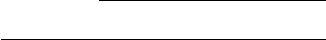
If the circular component is an arc, the points of intersection between the linear
component and circle must be tested to see if they are on the arc. Let the arc have
end points A and B, where the arc is that portion of the circle obtained by traversing
the circle counterclockwise from A to B. Notice that the line containing A and B
separates the arc from the remainder of the circle. Figure 7.1 illustrates this. If P
is a point on the circle, it is on the arc if and only if it is on the same side of that
line as the arc. The algebraic condition for the circle point P to be on the arc is
Kross(P − A, B −A) ≥ 0, where Kross((x
0
, y
0
), (x
1
, y
1
)) = x
0
y
1
− x
1
y
0
.
7.4 Linear Components and Polynomial Curves
Consider a line P + t
d for t ∈ R and a polynomial curve X(s) =
n
i=0
A
i
s
i
,where
A
n
=
0. Let the parameter domain be [s
min
, s
max
]. This section discusses how to
compute points of intersection between the line and curve from both an algebraic
and geometric perspective.
7.4.1 Algebraic Method
Intersections of the line and curve, if any, can be found by equating X(s) = P + t
d
and solving for s by eliminating the t-term using the Kross operator:
7.4 Linear Components and Polynomial Curves 249
B
P
A
C
R
Q
Figure 7.1 An arc of a circle spanned counterclockwise from A to B. The line containing A and
B separates the circle into the arc itself and the remainder of the circle. Point P is on
the arc since it is on the same side of the line as the arc. Point Q is not on the arc since
it is on the opposite side of the line.
n
i=0
Kross(
d,
A
i
)
s
i
= Kross(
d, X(s)) = Kross(
d, P + t
d) =Kross(
d, P)
Setting c
0
=Kross(
d,
A
0
−P)and c
i
=Kross(
d,
A
i
) for i ≥1, the previous equation
is reformulated as the polynomial equation q(s) =
n
i=0
c
i
s
i
= 0. A numerical root
finder can be applied to this equation, but beware of c
n
being zero (or nearly zero)
when
d and
A
n
are parallel (or nearly parallel). Any ¯s for which q(¯s) = 0 must be
tested for inclusion in the parameter domain [s
min
, s
max
]. If so, a point of intersection
has been found.
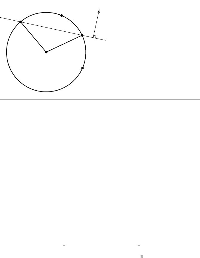
Example Let the line be (0, 1/2) + t(2, −1) and the polynomial curve be X(s) = (0, 0) +
s(1, 2) + s
2
(0, −3) + s
3
(0, 1) for s ∈ [0, 1]. The curve is unimodal and has x-range
[0, 1]and y-range [0, 3/8]. The polynomial equation is q(s) =2s
3
−6s
2
+5s −1 =0.
The roots are s =1, 1 ±
√
2/2. Only the roots 1 and 1 −
√
2/2 are in [0, 1]. Figure 7.2
shows the line, curve, and points of intersection
I
0
and
I
1
.
The numerical root finders might have problems finding roots of even multiplic-
ityoratarootwhereq(s) does not have a large derivative. Geometrically these cases
happen when the line and tangent line at the point of intersection form an angle that
is nearly zero.
Just as in the problem of computing intersections of linear components with
quadratic curves, if the application’s goal is to determine only if the linear component
and polynomial curve intersect, but does not care about where the intersections
250 Chapter 7 Intersection in 2D
Line
I
0
I
1
Curve
Figure 7.2 Intersection of a line and a cubic curve.
occur, then the root finding for q(s) = 0 can be skipped and Sturm sequences used
(Section A.5) to count the number of real-valued roots in the domain [s
min
, s
max
]
for the curve X(s). If the count is zero, then the line and polynomial curve do not
intersect.
Example Using the same example as the previous one, we only want to know the number of
real-valued roots for q(s) = 0 in [0, 1]. The Sturm sequence is q
0
(s) = 2s
3
− 6s
2
+
5s −1, q
1
(s) =6s
2
−12s +5, q
2
(s) =2(s −1)/3, and q
3
(s) =1. We have q
0
(0) =−1,
q
1
(0) = 5, q
2
(0) =−2/3, and q
3
(0) = 1 for a total of 3 sign changes. We also have
q
0
(1) = 0, q
1
(1) =−1, q
2
(1) = 0, and q
3
(1) = 1 for a total of 1 sign change. The
difference in sign changes is 2, so q(s) = 0 has two real-valued roots on [0, 1], which
means the line intersects the curve.
7.4.2 Polyline Approximation
The root finding of the algebraic method can be computationally expensive. An at-
tempt at reducing the time complexity is to approximate the curve by a polyline and
find intersections of the line with the polyline. The curve polyline is obtained by sub-
division (see Section A.8). The line-polyline tests that were discussed earlier in this
7.4 Linear Components and Polynomial Curves 251
chapter can be applied. Any intersections that are found can be used as approxima-
tions to line-curve intersections if the application is willing to accept that the polyline
is a suitable approximation to the curve. However, the points of intersection might be
used as an attempt to localize the search for actual points of intersection on the curve.
For example, if a line-polyline intersection occurred on the segment X(s
i
), X(s
i+1
),
the next step could be to search for a root of q(s) = 0 in the interval [s
i
, s
i+1)
].
7.4.3 Hierarchical Bounding
The algebraic method mentioned earlier always incurs the cost of root finding for a
polynomial equation. Presumably the worst case is that after spending the computer
time to find any real-valued roots of q(s) =0, there are none; the line and polynomial
curve do not intersect. An application might want to reduce the cost for determining
there is no intersection by providing coarser-level tests in hopes of an “early out”
from the intersection testing. Perhaps more important is that if the application will
perform a large number of line-curve intersection tests with different lines, but the
same curve, the total cost of polynomial root finding can be prohibitive. Some type
of curve preprocessing certainly can help to reduce the costs.
One coarse-level test involves maintaining a bounding polygon for the curve. In
particular, if the curve is built from control points and the curve lies in the convex hull
of the control points, an intersection test is first applied to the line and the convex hull
(a convex polygon). If they do not intersect, then the line and curve do not intersect. If
the line and polygon do intersect, then the application proceeds to the more expensive
line-curve test.
An alternative is to use an axis-aligned bounding rectangle for the curve. The
line-rectangle intersection test is quite inexpensive and is discussed in Section 7.7
on separating axes. If the application is willing to allow a few more cycles in hopes
of an early-out no-intersection test, a variation of the algorithm is to construct a
hierarchy of bounding boxes, each level providing a better fit (in some sense) than
the previous level. Moreover, if the line does not intersect a bounding box at some
level, then there is no point in processing further levels below the node of that box
since the line cannot intersect the curve in that localized region. Figure 7.3 illustrates
the idea. A curve is shown with a two-level hierarchy. The line intersects the top-level
box, so the next level of the hierarchy must be analyzed. The line intersects the left
child box at the next level, so further intersection tests are needed using either line-
box or line-curve tests. The line does not intersect the right child box at the next level,
so the line cannot intersect the curve contained in that box. No further processing of
that subtree of the hierarchy is needed.
The main question, of course, is how do you construct an axis-aligned bounding
box for a curve? For special classes of curves, specifically B
´
ezier curves, this is not dif-
ficult. An axis-aligned bounding box for the curve that is not usually of smallest area
is constructed for the control points of the curve. A hierarchy of boxes can be built by
subdividing the curve and fitting boxes to the control points that correspond to each

252 Chapter 7 Intersection in 2D
Left child
box
Right child box
Line
Top-level box
Curve
Figure 7.3 Line-curve intersection testing using a hierarchy of bounding boxes.
subcurve. For polynomial curves in general, finding the smallest-area axis-aligned
bounding box appears to be as complicated as the algorithm for finding intersections
of the line and the curve. The extent of the box in the x-direction is determined by
the x-extreme points on the curve. The x-extreme points are characterized by hav-
ing vertical tangents to the curve. Mathematically, (x(t), y(t)) has a vertical tangent
if x
(t) = 0. Similarly, the y-extreme points are characterized by having horizontal
tangents to the curve where y
(t) =0. Each derivative equation is a polynomial equa-
tion that can be solved by numerical methods, but proceeding this way invalidates
the goal of using a bounding box to avoid expensive root finding in regions where the
line does not intersect the curve. This might not be an issue if the original curve is cu-
bic, in which case the derivative equations can be solved using the quadratic formula.
This is also not an issue if the application plans on testing for intersections between
multiple lines and a single curve. The preprocessing costs for computing a bound-
ing box are negligible compared to the total costs of root finding for the line-curve
intersection tests.
7.4.4 Monotone Decomposition
Now suppose that x
(t) = 0 for any t ∈ [t
min
, t
max
]. The curve is monotonic in x,ei-
ther strictly increasing or strictly decreasing. In this special case, the x-extents for
the axis-aligned bounding box correspond to x(t
min
) and x(t
max
). A similar argu-
ment applies if y
(t) = 0 on the curve domain. Generally, if x
(t) = 0 and y
(t) = 0
for t ∈[a, b]⊆[t
min
, t
max
], then the curve segment is monotonic and the axis-aligned
bounding box is determined by the points (x(a), y(a)) and (x(b), y(b)). Determin-
ing that a derivative equation does not have roots is an application of Sturm se-
quences, as discussed in Section A.5.
7.4 Linear Components and Polynomial Curves 253
The idea now is to subdivide the curve using a simple bisection on the parameter
interval with the goal of finding monotonic curve segments. If [a, b] is a subinterval
in the bisection for which the curve is monotonic, no further subdivision occurs; the
axis-aligned bounding box is known for that segment. Ideally, after a few levels of
bisection we obtain a small number of monotonic segments and their corresponding
bounding boxes. The line-box intersection tests can be applied between the line and
each box in order to cull out monotone segments that do not intersect the line, but if
the number of boxes is large, you can always build a hierarchy from the bottom up by
treating the original boxes as leaf nodes of a tree, then grouping a few boxes at a time
to construct parent nodes. The bounding box of a parent node can be computed to
contain the bounding boxes of its children. The parents themselves can be grouped,
the process eventually leading to the root node of the tree with a single bounding box.
The method of intersection illustrated in Figure 7.3 may be applied to this tree.
A recursive subdivision may be applied to find monotone segments. The recur-
sion requires a stopping condition that should be chosen carefully. If the derivative
equations x
(t) = 0 and y
(t) = 0 both indicate zero root counts on the current in-
terval, then the curve is monotonic on that interval and the recursion terminates. If
one of the equations has a single root on the current interval and the other does not,
a subdivision is applied. It is possible that the subdivision t-value is the root itself,
in which case both subintervals will report a root when there is only a single root.
For example, consider (x(t), y(t)) = (t , t
2
) for t ∈ [−1, 1]. The derivative equation
x
(t) = 0 has no solution since x
(t) = 1 for all t, but y
(t) = 2t = 0hasonerooton
the interval. The subdivision value is t = 0. The equation y
(t) = 0hasonerooton
the subinterval [−1, 0] and one root on the subinterval [0, 1], but these are the same
root. The end points of subintervals should be checked to avoid deeper recursions
than necessary. The typical case, though, is that a root of a subinterval occurs in the
interior of the interval. Once a subinterval that has a single interior root is found, a
robust bisection can be applied to find the root and subdivide the subinterval at the
root. The recursion terminates for that subinterval.
In an application that will perform intersection queries with multiple lines but
only one curve, the monotone segments can be found as a preprocessing step by
solving x
(t) = 0 and y
(t) = 0 using numerical root finders.
7.4.5 Rasterization
A raster approach may be used, even though it is potentially quite expensive to
execute. An axis-aligned bounding box [x
min
, x
max
] × [y
min
, y
max
] is constructed to
contain the curve. An N × M raster is built to represent the box region. The grid
points are uniformly chosen as (x
i
, y
j
) for 0 ≤ i<Nand 0 ≤j<M. That is, x
i
=
x
min
+ (x
max
− x
min
)i/(N − 1) and y
j
= y
min
+ (y
max
− y
min
)j/(M − 1). Both the
line and the curve are drawn into the raster. The step size for the parameter of the
curve should be chosen to be small enough so that as the curve is sampled you
generate adjacent raster values, potentially with a raster cell drawn multiple times