Schneider P., Eberly D.H. Geometric Tools for Computer Graphics
Подождите немного. Документ загружается.

254 Chapter 7 Intersection in 2D
Contains line
Contains curve
Contains both
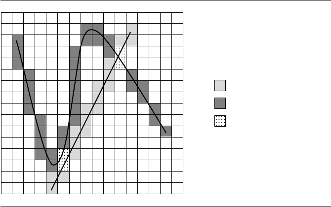
Figure 7.4 A line and a curve rasterized on a grid that is initially zero. The line is rasterized by
or-ing the grid with the mask 1 (light gray). The curve is rasterized by or-ing the grid
with the mask 2 (dark gray). Grid cells that contain both the line and the curve have
a value 3 (dotted).
because multiple curve samples fall inside that cell. The overdraw can be reduced by
sampling the curve based on arc length rather than the curve parameter. If the raster is
initialized with 0, the line is drawn by or-ing the pixels with 1, and the curve is drawn
by or-ing the pixels with 2. The pixels that are associated with line-curve intersections
are those with a final value of 3. Figure 7.4 illustrates this.
The effectiveness of this method depends on how well the grid cell size is chosen.
If it is chosen to be too large, the line and curve can pass through the same pixel, yet
not intersect. The rasterization method reports an intersection when there is none.
This situation is shown in Figure 7.4 in the lower-left portion of the grid. If the cell
size is chosen to be too small, a lot of time is consumed in rasterizing the curve,
especially in pixels that the line does not intersect.
Just as in the polyline approach, the application can choose to accept the pixel
values as approximations to the actual line-curve intersections. If more accuracy is
desired, the pixels tagged as 3 (and possibly immediate neighbors) can be used as
a localization of where the intersections occur. If a contiguous block of pixels is
tagged, such as is shown in the upper right of the grid in Figure 7.4, and if the
application chooses to believe the block occurs because of a single intersection of
curves, a suitable choice for the approximation is the average of pixel locations. If
the application chooses not to accept the pixel values as approximations, then it can

7.5 Quadratic Curves 255
store the original line and curve parameters for samples occurring in a pixel with that
pixel. Those parameter values can be used to start a search for intersections using a
numerical root finder or a numerical distance calculator.
7.5 Quadratic Curves
We present a general algebraic method for computing intersection points between
two curves defined implicitly by quadratic curves. The special case of circular com-
ponents is also presented because it handles intersection between circular arcs. Vari-
ations on computing intersection points of two ellipses are also presented here as an
illustration of how you might go about handling the more general problem of inter-
section between two curves, each defined as a level curve for a particular function.
7.5.1 General Quadratic Curves
Given two curves implicitly defined by the quadratic equations F(x, y) = α
00
+
α
10
x + α
01
y + α
20
x
2
+ α
11
xy + α
02
y
2
= 0 and G(x, y) = β
00
+ β
10
x + β
01
y+
β
20
x
2
+ β
11
xy + β
02
y
2
= 0, the points of intersection can be computed by elim-
inating y to obtain a fourth-degree polynomial equation H(x) = 0. During the
elimination process, y is related to x via a rational polynomial equation, y = R(x).
Each root ¯x of H(x)= 0 is used to compute ¯y =R(¯x). The pair ( ¯x, ¯y) is an intersec-
tion point of the two original curves.
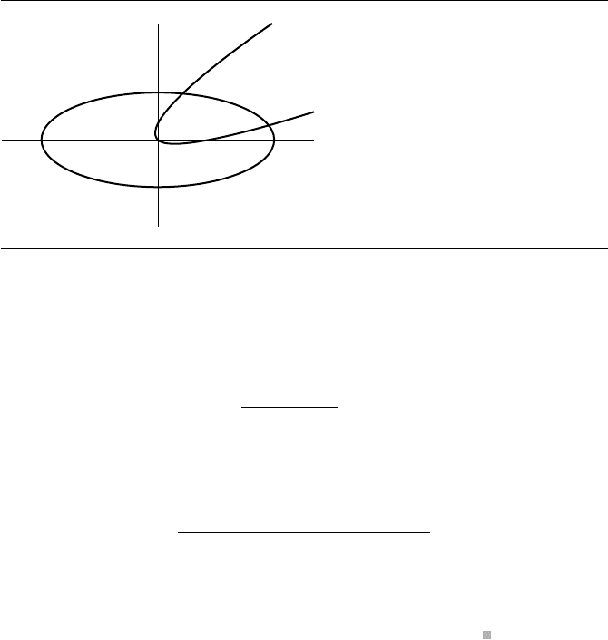
Example The equation x
2
+ 6y
2
− 1 = 0 defines an ellipse whose center is at the origin. The
equation 2(x −2y)
2
−(x +y) =0 determines a parabola whose vertex is the origin.
Figure 7.5 shows the plots of the two curves. The ellipse equation is rewritten as
y
2
= (1 − x
2
)/6. Substituting this in the parabola equation produces
0 =2x
2
− 8xy + 8y
2
− x − y = 2x
2
− 8xy + 8(1 − x
2
)/6 −x − y
=−(8x + 1)y +(2x
2
− 3x + 4)/3
This may be solved for
y =
2x
2
− 3x + 4
3(8x +1)
=: R(x)
Replacing this in the ellipse equation produces
256 Chapter 7 Intersection in 2D
–1 1
–0.408
0.408
Figure 7.5 Intersections of an ellipse and a parabola.
0 =x
2
+ 6y
2
− 1
= x
2
+ 6
2x
2
− 3x + 4
3(8x +1)
2
− 1
=
9(8x + 1)
2
(x
2
− 1) + 6(2x
2
− 3x + 4)
2
9(8x + 1)
2
=
200x
4
+ 24x
3
− 139x
2
− 96x +29
3(8x +1)
2
Therefore, it is necessary that
0 =200x
4
+ 24x
3
− 139x
2
− 96x +29 =: H(x)
The polynomial equation H(x) = 0 has two real-valued roots, x
0
.
=
0.232856
and x
1
.
=
0.960387. Replacing these in the rational polynomial for y produces y
0
=
R(x
0
)
.
=
0.397026 and y
1
=R(x
1
)
.
=
0.113766. The points (x
0
, y
0
) and (x
1
, y
1
) are the
intersection points for the ellipse and parabola.
The general method of solution of two polynomial equations is discussed in detail
in Section A.2.
As with any root finder, numerical problems can arise when a root has even mul-
tiplicity or the derivative of the function near the root is small in magnitude. These
problems tend to arise geometrically when the two curves have an intersection point
for which the angle between tangent lines to the curves at the point is nearly zero.
If you need extreme accuracy and do not want to miss intersection points, you will
need your root finder to be quite robust at the expense of some extra computational
time.
7.5 Quadratic Curves 257
If the application only needs to know if the curves intersect, but not where, then
the method of Sturm sequences for root counting can be applied to H(x) = 0. The
method is discussed in Section A.5.
7.5.2 Circular Components
Let the two circles be represented by X − C
i
2
= r
2
i
for i = 0, 1. The points of
intersection, if any, are determined by the following construction. Define u = C
1
−
C
0
=(u
0
, u
1
). Define v =(u
1
, −u
0
). Note that u
2
=v
2
=C
1
−C
0
2
and u ·v =
0. The intersection points can be written in the form
X = C
0
+ s u + t v (7.1)
or
X = C
1
+ (s − 1)u + t v (7.2)
where s and t are constructed by the following argument. Substituting Equation 7.1
into X − C
0
2
= r
2
0
yields
(s
2
+ t
2
)u
2
= r
2
0
(7.3)
Substituting Equation 7.2 into X − C
1
2
= r
2
1
yields
((s −1)
2
+ t
2
)u
2
= r
2
1
(7.4)
Subtracting Equations 7.3 and 7.4 and solving for s yields
s =
1
2
r
2
0
− r
2
1
u
2
+ 1
(7.5)
Replacing Equation 7.5 into Equation 7.3 and solving for t
2
yields
t
2
=
r
2
0
u
2
− s
2
=
r
2
0
u
2
−
1
4
r
2
0
− r
2
1
u
2
+ 1
2
=−
(u
2
− (r
0
+ r
1
)
2
)(u
2
− (r
0
− r
1
)
2
)
4u
4
(7.6)
In order for there to be solutions, the right-hand side of Equation 7.6 must be non-
negative. Therefore, the numerator is negative:
(u
2
− (r
0
+ r
1
)
2
)(u
2
− (r
0
− r
1
)
2
) ≤ 0 (7.7)
258 Chapter 7 Intersection in 2D
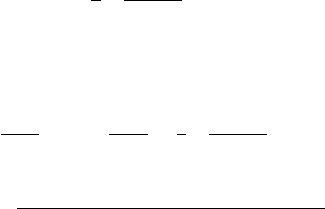
(c)
R
0
R
1
C
0
C
1
(a) (b)
Figure 7.6 Relationship of two circles, u = C
1
− C
0
: (a) u=|r
0
+ r
1
|; (b) u=|r
0
− r
1
|;
(c) |r
0
− r
1
| < u < |r
0
+ r
1
|.
If w =u, the left-hand side of Inequality 7.7 defines a quadratic function of
w, the graph being a parabola that opens upwards. The roots are w =|r
0
− r
1
| and
w =|r
0
+r
1
|. For the quadratic function to be negative, only values of w between the
two roots are allowed. Inequality 7.7 is therefore equivalent to
|r
0
− r
1
|≤u≤|r
0
+ r
1
| (7.8)
If u=|r
0
+r
1
|, each circle is outside the other circle, but just tangent. The point
of intersection is C
0
+ (r
0
/(r
0
+ r
1
))u.Ifu=|r
0
− r
1
|, the circles are nested and
just tangent. The circles are the same if u=0 and r
0
= r
1
; otherwise the point of
intersection is C
0
+(r
0
/(r
0
−r
1
))u.If|r
0
−r
1
|< u< |r
0
+r
1
|, then the two circles
intersect in two points. The s-value from Equation 7.5 and the t-values from taking
the square root in Equation 7.6 can be used to compute the intersection points as
C
0
+ s u + t v. Figure 7.6 shows the various relationships for the two circles.
If either or both circular components are arcs, the circle-circle points of intersec-
tion must be tested if they are on the arc (or arcs) using the circular-point-on-arc test
described earlier in this chapter.
7.5.3 Ellipses
The algebraic method discussed earlier for testing/finding points of intersection ap-
plies, of course, to ellipses since they are implicitly defined by quadratic equations.
In some applications, more information is needed other than just knowing points of
intersection. Specifically, if the ellipses are used as bounding regions, it might be im-
portant to know if one ellipse is fully contained in another. This information is not
provided by the algebraic method applied to the two quadratic equations defining the
ellipses. The more precise queries for ellipses E
0
and E
1
are
Do E
0
and E
1
intersect?
Are E
0
and E
1
separated? That is, does there exist a line for which the ellipses are
on opposite sides?
Is E
0
properly contained in E
1
,orisE
1
properly contained in E
0
?
7.5 Quadratic Curves 259
Q
0
> 0
Q
0
< 0
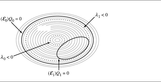
Figure 7.7 E
1
is contained in E
0
. The maximum E
0
level curve value λ
1
for E
1
is negative.
Let the ellipse E
i
be defined by the quadratic equation Q
i
(X) = X
T
A
i
X +
B
T
i
X + c
i
for i = 0, 1. It is assumed that the A
i
are positive definite. In this case,
Q
i
(X) < 0 defines the inside of the ellipse, and Q
i
(X) > 0 defines the outside.
The discussion focuses on level curves of the quadratic functions. Section A.9.1
provides a discussion of level sets of functions. All level curves defined by Q
0
(x, y) =
λ are ellipses, except for the minimum (negative) value λ for which the equation
defines a single point, the center of every level curve ellipse. The ellipse defined by
Q
1
(x, y) =0 is a curve that generally intersects many level curves of Q
0
. The problem
is to find the minimum level value λ
0
and maximum level value λ
1
attained by any
(x, y) on the ellipse E
1
.Ifλ
1
< 0, then E
1
is properly contained in E
0
.Ifλ
0
> 0,
then E
0
and E
1
are separated or E
1
contains E
0
. Otherwise, 0 ∈ [λ
0
, λ
1
] and the two
ellipses intersect. Figures 7.7, 7.8, and 7.9 illustrate the three possibilities. The figures
show the relationship of one ellipse E
1
to the level curves of another ellipse E
0
.
This can be formulated as a constrained optimization that can be solved by the
method of Lagrange multipliers (see Section A.9.3): Optimize Q
0
(X) subject to the
constraint Q
1
(X) = 0. Define F(X, t) = Q
0
(X) + tQ
1
(X). Differentiating with re-
spect to the components of X yields
∇F =
∇Q
0
+t
∇Q
1
. Differentiating with respect
to t yields ∂F /∂t = Q
1
. Setting the t-derivative equal to zero reproduces the con-
straint Q
1
= 0. Setting the X-derivative equal to zero yields
∇Q
0
+ t
∇Q
1
=
0 for
some t. Geometrically this means that the gradients are parallel.
Note that
∇Q
i
= 2A
i
X + B
i
,so
0 =
∇Q
0
+ t
∇Q
1
= 2(A
0
+ tA
1
)X + (B
0
+ tB
1
)
Formally solving for X yields
260 Chapter 7 Intersection in 2D
Q
0
> 0
Q
0
< 0
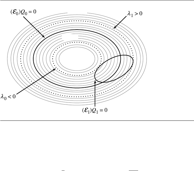
Figure 7.8 E
1
transversely intersects E
0
. The minimum E
0
level curve value λ
0
for E
1
is negative;
the maximum value λ
1
is positive.
X =−
1
2
(A
0
+ tA
1
)
−1
(B
0
+ tB
1
) =
1
δ(t)
Y(t)
where A
0
+ tA
1
is a matrix of linear polynomials in t and δ(t) is its determinant,
a quadratic polynomial. The components of
Y(t) are quadratic polynomials in t.
Replacing this in Q
1
(X) = 0 yields
p(t) :=
Y(t)
T
A
1
Y(t)+ δ(t)B
T
1
Y(t)+ δ(t)
2
C
1
= 0 (7.9)
a quartic polynomial in t. The roots can be computed, the corresponding values of X
computed, and Q
0
(X) evaluated. The minimum and maximum values are stored as
λ
0
and λ
1
, and the earlier comparisons with zero are applied.
This method leads to a quartic polynomial, just as the original algebraic method
for finding intersection points did. But the current style of query does answer ques-
tions about the relative positions of the ellipses (separated or proper containment)
whereas the original method does not.
Example Consider Q
0
(x, y) = x
2
+ 6y
2
− 1 and Q
1
(x, y) = 52x
2
− 72xy + 73y
2
− 32x −
74y +28. Figure 7.10 shows the plots of the two ellipses. The various parameters are
7.5 Quadratic Curves 261
Q
0
< 0
Q
0
> 0
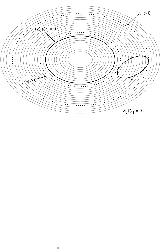
Figure 7.9
E
1
is separated from E
0
. The minimum E
0
level curve value λ
0
for E
1
is positive.
A
0
=
10
06
, B
0
=
0
0
, C
0
=−1, A
1
=
52 −36
−36 73
,
B
1
=
−32
−74
, C
1
= 28
From these are derived
Y(t)=
4t(625t + 24)
t(2500t + 37)
, δ(t) = 2500t
2
+ 385t + 6
The polynomial of Equation 7.9 is p(t) =−156250000t
4
− 48125000t
3
+
1486875t
2
+ 94500t + 1008. The two real-valued roots are t
0
.
=
−0.331386 and t
1
.
=
0.0589504. The corresponding X(t) values are X(t
0
) = (x
0
, y
0
)
.
=
(1.5869, 1.71472)
and X(t
1
) = (x
1
, y
1
)
.
=
(0.383779, 0.290742). The axis-aligned ellipse level values at
these points are Q
0
(x
0
, y
0
) =−0.345528 and Q
0
(x
1
, y
1
) = 19.1598. Since Q
0
(x
0
, y
0
)
< 0 <Q
0
(x
1
, y
1
), the ellipses intersect. Figure 7.10 shows the two points on Q
1
= 0
that have extreme Q
0
values.
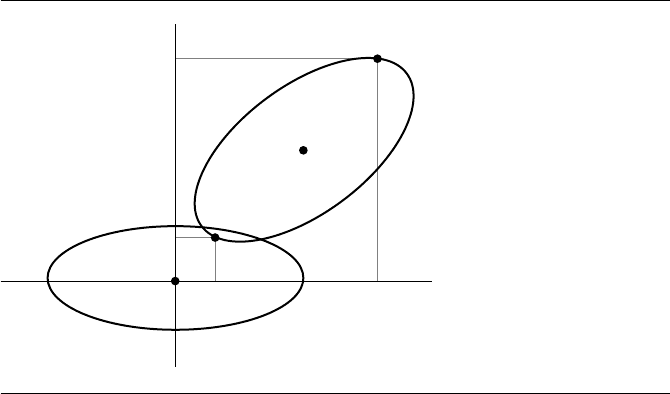
262 Chapter 7 Intersection in 2D
1.71
0.408
0.38
–0.408
–1 1 1.580.29
Figure 7.10 Intersection of two ellipses.
7.6 Polynomial Curves
Consider two polynomial curves, X(s) =
n
i=0
A
i
s
i
,where
A
n
=
0 and s ∈
[s
min
, s
max
], and Y(t)=
m
j=0
B
j
t
j
,where
B
m
=
0 and t ∈ [t
min
, t
max
]. This section
discusses how to compute points of intersection between the curves from both an
algebraic and geometric perspective.
7.6.1 Algebraic Method
The straightforward algebraic method is to equate X(s) = Y(t) and solve for the
parameters s and t. Observe that the vector equation yields two polynomial equations
of degree max{n, m}in the two unknowns s and t. The method of elimination may be
used to obtain a single polynomial equation in one variable, q(s) = 0. The method
of solution is a simple extension to what was shown in the section on intersection
finding for lines and polynomial curves, except that the degree of q(s) will be larger
than in that case (for the line, m = 1; for curves, we generally have m>1).
7.6.2 Polyline Approximation
The root finding of the algebraic method can be computationally expensive. Simi-
lar to Section 7.4 for line-curve intersection testing, the time complexity is reduced
7.6 Polynomial Curves 263
by approximating both curves by polylines and finding intersections of the two
polylines. The polylines are obtained by subdivision, described in Section A.8. Any
intersections between the polylines can be used as approximations to curve-curve
intersections if the application is willing to accept that the polylines are suitable ap-
proximations to the curves. However, the points of intersection might be used as an
attempt to localize the search for actual points of intersection.
7.6.3 Hierarchical Bounding
In Section 7.4 we discussed using coarse-level testing using bounding polygons,
bounding boxes, or hierarchies of bounding boxes to allow for an early out when
the two underlying objects do not intersect. The same ideas apply to curve-curve
intersection testing. If the curves are defined by control points and have the convex
hull property, then an early-out algorithm would test first to see if the convex poly-
gons containing the curves intersect. If not, then the curves do not intersect. If so, a
finer-level test is used, perhaps directly the algebraic method described earlier.
A hierarchical approach using box trees can also be used. Each curve has a box
hierarchy constructed for it. To localize the intersection testing, pairs of boxes, one
from each tree, must be compared. This is effectively the 3D-oriented bounding box
approach used by Gottschalk, Lin, and Manocha (1996), but in 2D and applied to
curve segments instead of polylines. One issue is to perform an amortized analysis
to determine at what point the box-box intersection tests become more expensive
than the algebraic method for curve-curve intersection tests. At that point the sim-
plicity of box-box intersection tests is outweighed by its excessive cost. A lot of the
cost is strongly dependent on how deep the box hierarchies are. Another issue is
construction of axis-aligned bounding boxes for curves. This was discussed in Sec-
tion 7.4.
7.6.4 Rasterization
Finally, a raster approach may be used, even though it is potentially quite expensive
to execute. An axis-aligned bounding box [x
min
, x
max
] × [y
min
, y
max
] is constructed
to contain both curves. An N × M raster is built to represent the box region. The
grid points are uniformly chosen as (x
i
, y
j
) for 0 ≤ i<Nand 0 ≤ j<M. That is,
x
i
=x
min
+(x
max
−x
min
)i/(N −1) and y
j
=y
min
+(y
max
−y
min
)j/(M −1).Each
curve is drawn into the raster. The step size for the parameter of the curve should be
chosen to be small enough so that as the curve is sampled you generate adjacent raster
values, potentially with a raster cell drawn multiple times because multiple curve
samples fall inside that cell. The overdraw can be minimized by sampling the curve
based on arc length rather than the curve parameter. If the raster is initialized with
0, the first curve drawn by or-ing the pixels with 1, and the second curve drawn by