Smith R., Minton R. Calculus
Подождите немного. Документ загружается.

P1: OSO/OVY P2: OSO/OVY QC: OSO/OVY T1: OSO
MHDQ256-Ch00 MHDQ256-Smith-v1.cls December 8, 2010 15:25
LT (Late Transcendental)
CONFIRMING PAGES
0-23 SECTION 0.3
..
Graphing Calculators and Computer Algebra Systems 23
y
x
y a
3
x
3
a
2
x
2
a
1
x a
0
Inflection
point
FIGURE 0.33b
Cubic: no max or min, a
3
< 0
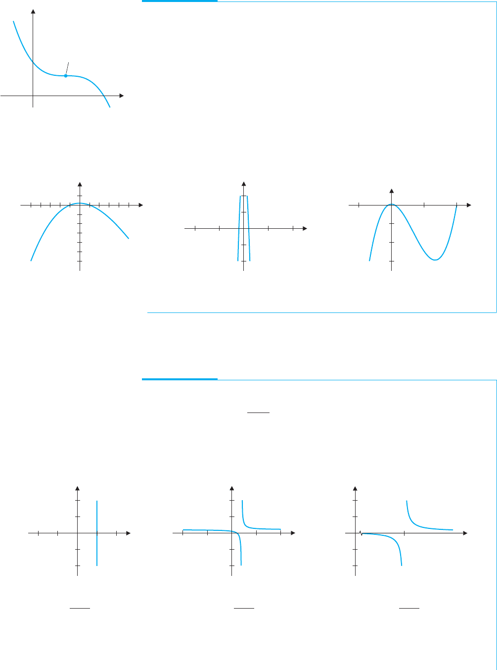
EXAMPLE 3.2 Sketching the Graph of a Cubic Polynomial
Sketch a graph of the cubic polynomial f (x) = x
3
− 20x
2
− x +20.
Solution Your initial graph probably looks like Figure 0.34a or 0.34b.
However, you should recognize that neither of these graphs looks like a cubic; they
look more like parabolas. To see the S-shape behavior in the graph, we need to consider
a larger range of x-values. To determine how much larger, we need some of the concepts
of calculus. For the moment, we use trial and error, until the graph resembles the shape
of a cubic. You should recognize the characteristic shape of a cubic in Figure 0.34c.
Although we now see more of the big picture (often referred to as the global behavior
of the function), we have lost some of the details (such as the x-intercepts), which we
could clearly see in Figures 0.34a and 0.34b (often referred to as the local behavior of
the function).
x
44
200
400
600
y
y
x
105510
10
10
x
10
20
10
800
400
1200
y
FIGURE 0.34a
f (x) = x
3
− 20x
2
− x + 20
FIGURE 0.34b
f (x) = x
3
− 20x
2
− x + 20
FIGURE 0.34c
f (x) = x
3
− 20x
2
− x + 20
Rational functions have some properties not found in polynomials, as we see in
examples 3.3, 3.4 and 3.5.
EXAMPLE 3.3 Sketching the Graph of a Rational Function
Sketch a graph of f (x) =
x −1
x −2
and describe the behavior of the graph near x = 2.
Solution Your initial graph should look something like Figure 0.35a or 0.35b. From
either graph, it should be clear that something unusual is happening near x = 2.
Zooming in closer to x = 2 should yield a graph like that in Figure 0.35c.
y
x
44
1e08
5e07
5e07
1e08
y
x
105510
10
5
5
10
y
2
20
10
10
20
x
FIGURE 0.35a
y =
x − 1
x − 2
FIGURE 0.35b
y =
x − 1
x − 2
FIGURE 0.35c
y =
x − 1
x − 2
In Figure 0.35c, it appears that as x increases up to 2, the function values get more
and more negative, while as x decreases down to 2, the function values get more and
more positive. (Note that the notation used for the y-axis labels is the exponential form
P1: OSO/OVY P2: OSO/OVY QC: OSO/OVY T1: OSO
MHDQ256-Ch00 MHDQ256-Smith-v1.cls December 8, 2010 15:25
LT (Late Transcendental)
CONFIRMING PAGES
24 CHAPTER 0
..
Preliminaries 0-24
used by many graphing utilities, where 5e + 07 corresponds to 5 × 10
7
.) This is also
observed in the following table of function values.
x f(x)
1.8 −4
1.9 −9
1.99 −99
1.999 −999
1.9999 −9999
x f(x)
2.2 6
2.1 11
2.01 101
2.001 1001
2.0001 10,001
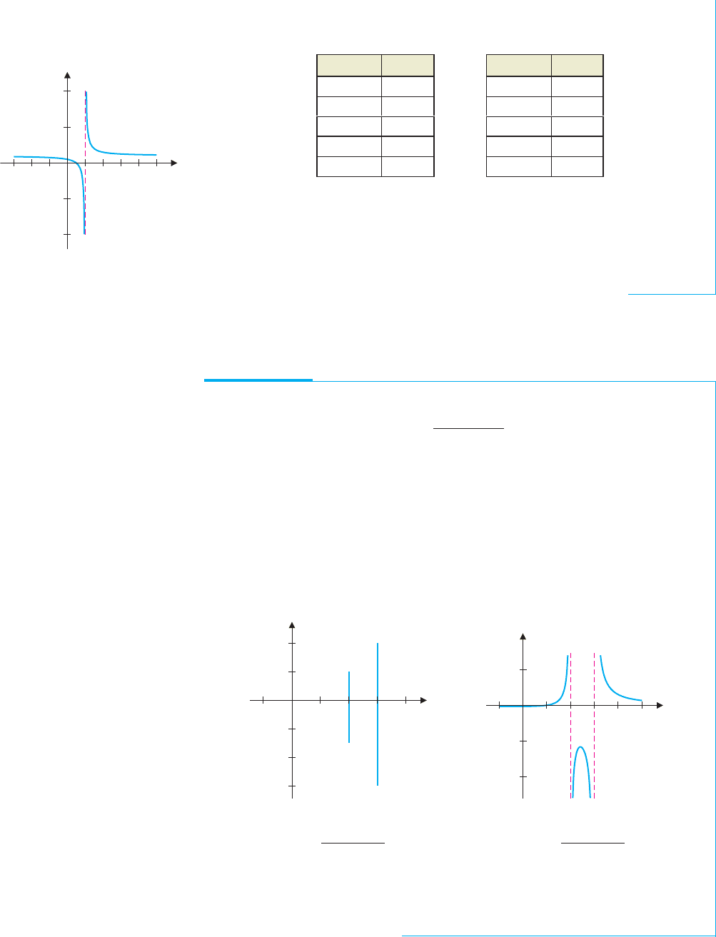
Note that at x = 2, f (x) is undefined. However, as x approaches 2 from the left, the
graph veers down sharply. In this case, we say that f (x) tends to −∞. Likewise, as x
approaches 2 from the right, the graph rises sharply. Here, we say that f (x) tends to
∞ and there is a vertical asymptote at x = 2. (We’ll define this more carefully in
Chapter 1.) It is common to draw a vertical dashed line at x = 2 to indicate this. (See
Figure 0.36.) Since f (2) is undefined, there is no point plotted at x = 2.
y
x
484
10
5
5
10
FIGURE 0.36
Vertical asymptote
Many rational functions have vertical asymptotes. You can locate possible vertical
asymptotes by finding where the denominator is zero. It turns out that if the numerator is
not zero at that point, there is a vertical asymptote at that point.
EXAMPLE 3.4 A Graph with More Than One Vertical Asymptote
Find all vertical asymptotes for f (x) =
x −1
x
2
− 5x + 6
.
Solution Note that the denominator factors as
x
2
− 5x + 6 = (x −2)(x −3),
so that the only possible locations for vertical asymptotes are x = 2 and x = 3. Since
neither x-value makes the numerator (x − 1) equal to zero, there are vertical asymptotes
at both x = 2 and x = 3. A computer-generated graph gives little indication of how the
function behaves near the asymptotes. (See Figure 0.37a and note the scale on the
y-axis.)
y
x
1 4
3e08
2e08
1e08
1e08
2e08
y
x
4 51
10
5
5
FIGURE 0.37a
y =
x − 1
x
2
− 5x + 6
FIGURE 0.37b
y =
x − 1
x
2
− 5x + 6
We can improve the graph by zooming-in in both the x- and y-directions.
Figure 0.37b shows a graph of the same function using the graphing window defined by
the rectangle −1 ≤ x ≤ 5 and −13 ≤ y ≤ 7. This graph clearly shows the vertical
asymptotes at x = 2 and x = 3.
As we see in example 3.5, not all rational functions have vertical asymptotes.
P1: OSO/OVY P2: OSO/OVY QC: OSO/OVY T1: OSO
MHDQ256-Ch00 MHDQ256-Smith-v1.cls December 8, 2010 15:25
LT (Late Transcendental)
CONFIRMING PAGES
0-25 SECTION 0.3
..
Graphing Calculators and Computer Algebra Systems 25
EXAMPLE 3.5 A Rational Function with No Vertical Asymptotes
Find all vertical asymptotes of f (x) =
x −1
x
2
+ 4
.
Solution Notice that x
2
+ 4 = 0 has no (real) solutions, since x
2
+ 4 > 0 for all
real numbers, x. So, there are no vertical asymptotes. The graph in Figure 0.38 is
consistent with this observation.
y
x
201010
0.2
0.2
0.4
FIGURE 0.38
y =
x − 1
x
2
+ 4
Graphs are useful for finding approximate solutions of difficult equations, as we see in
examples 3.6 and 3.7.
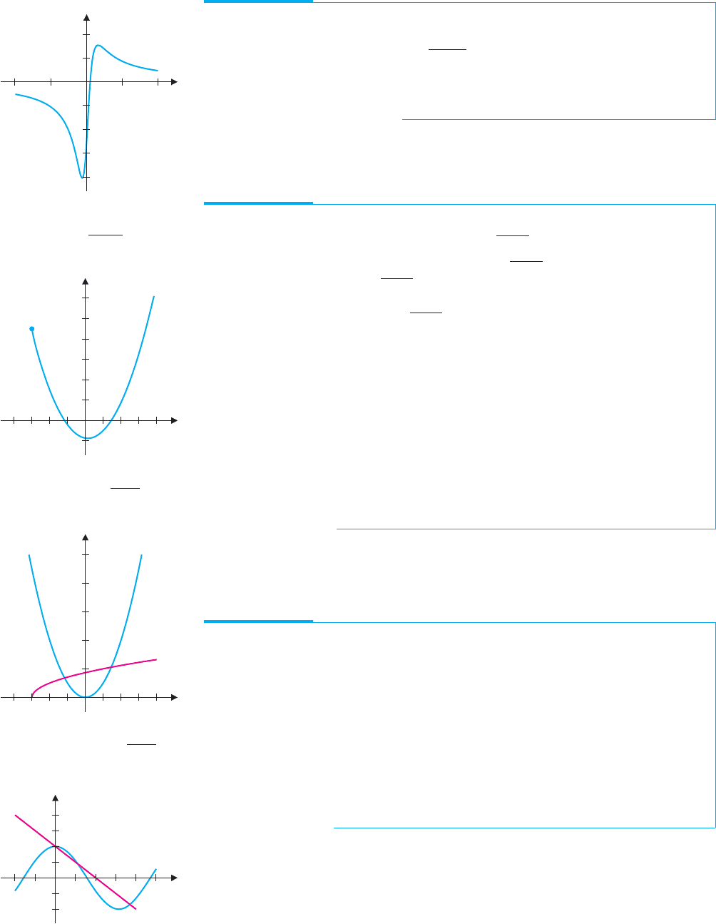
EXAMPLE 3.6 Finding Zeros Approximately
Find approximate solutions of the equation x
2
=
√
x +3.
Solution You could rewrite this equation as x
2
−
√
x +3 = 0 and then look for zeros
in the graph of f (x) = x
2
−
√
x +3, seen in Figure 0.39a. Note that two zeros are
clearly indicated: one near −1, the other near 1.5. However, since you know very little
of the nature of the function x
2
−
√
x +3, you cannot say whether or not there are any
zeros that don’t show up in the window seen in Figure 0.39a. On the other hand, if you
graph the two functions on either side of the equation on the same set of axes, as in
Figure 0.39b, you can clearly see two points where the graphs intersect (corresponding
to the two zeros seen in Figure 0.39a). Further, since you know the general shapes of
both of the graphs, you can infer from Figure 0.39b that there are no other intersections
(i.e., there are no other zeros of f ). This is important information that you cannot obtain
from Figure 0.39a. Now that you know how many solutions there are, you need to
estimate their values. One method is to zoom in on the zeros graphically. We leave it as
an exercise to verify that the zeros are approximately x = 1.4 and x =−1.2. If your
calculator or computer algebra system has a solve command, you can use it to quickly
obtain an accurate approximation. In this case, we get x ≈ 1.452626878 and
x ≈−1.164035140.
y
x
2 424
4
8
12
FIGURE 0.39a
y = x
2
−
√
x + 3
y
x
2 424
4
6
8
2
10
FIGURE 0.39b
y = x
2
and y =
√
x + 3
y
x
1 3 51
2
4
FIGURE 0.40
y = 2 cos x and y = 2 − x
When using the solvecommand on your calculator or computer algebra system, be sure
to check that the solutions make sense. If the results don’t match what you’ve seen in your
preliminarysketches,beware! Evenhigh-techequation solversmakemistakes occasionally.
EXAMPLE 3.7 Finding Intersections by Calculator: An Oversight
Find all points of intersection of the graphs of y = 2cos x and y = 2 − x.
Solution Notice that the intersections correspond to solutions of the equation
2cos x = 2 − x. Using the solve command on one graphing calculator, we found
intersections at x ≈ 3.69815 and x = 0. So, what’s the problem? A sketch of the graphs
of y = 2 − x and y = 2cos x (we discuss this function in the next section) clearly
shows three intersections. (See Figure 0.40.)
The middle solution, x ≈ 1.10914, was somehow passed over by the calculator’s
solve routine. The lesson here is to use graphical evidence to support your solutions,
especially when using software and/or functions with which you are less than
completely familiar.
You need to look skeptically at the answers provided by your calculator’s solver pro-
gram. While such solvers provide a quick means of approximating solutions of equations,
these programs will sometimes overlook solutions, as we saw in example 3.7, or return
incorrect answers, as we illustrate with example 3.8. So, how do you know if your solver is
giving you an accurate answer or one that’s incorrect? The only answer to this is that you
must carefully test your calculator’s solution, by separately calculating both sides of the
equation (by hand) at the calculated solution.

P1: OSO/OVY P2: OSO/OVY QC: OSO/OVY T1: OSO
MHDQ256-Ch00 MHDQ256-Smith-v1.cls December 8, 2010 15:25
LT (Late Transcendental)
CONFIRMING PAGES
26 CHAPTER 0
..
Preliminaries 0-26
EXAMPLE 3.8 Solving an Equation by Calculator: An Erroneous Answer
Use your calculator’s solver program to solve the equation x +
1
x
=
1
x
.
Solution Certainly, you don’t need a calculator to solve this equation, but consider
what happens when you use one. Most calculators report a solution that is very close to
zero, while others report that the solution is x = 0. Not only are these answers
incorrect, but the given equation has no solution, as follows. First, notice that the
equation makes sense only when x = 0. Subtracting
1
x
from both sides of the equation
leaves us with x = 0, which can’t possibly be a solution, since it does not satisfy the
original equation. Notice further that, if your calculator returns the approximate solution
x = 1 ×10
−7
and you use your calculator to compute the values on both sides of the
equation, the calculator will compute
x +
1
x
= 1 × 10
−7
+ 1 ×10
7
,
which it approximates as 1 × 10
7
=
1
x
, since calculators carry only a finite number of
digits. In other words, although
1 × 10
−7
+ 1 ×10
7
= 1 × 10
7
,
your calculator treats these numbers as the same and so incorrectly reports that the
equation is satisfied. The moral of this story is to be an intelligent user of technology
and don’t blindly accept everything your calculator tells you.
Wewanttoemphasizeagainthatgraphingshouldbethefirststepintheequation-solving
process. A good graph will show you how many solutions to expect, as well as give their
approximate locations. Whenever possible, you should factor or use the quadratic formula
to get exact solutions. When this is impossible, approximate the solutions by zooming in
on them graphically or by using your calculator’s solve command. It is helpful to compare
your results to a graph to see if there’s anything you’ve missed.
EXERCISES 0.3
WRITING EXERCISES
1. Explain why there is a significant difference among Fig-
ures 0.34a, 0.34b and 0.34c.
2. In Figure 0.36, the graph approaches the lower portion of the
verticalasymptote from the left, whereas the graph approaches
the upper portion of the vertical asymptote from the right. Use
thetableoffunctionvaluesfoundinexample3.3toexplainhow
to determine whether a graph approaches a vertical asymptote
by dropping down or rising up.
3. In the text, we discussed the difference between graphing
with a fixed window versus an automatic window. Discuss the
advantagesanddisadvantagesof each. (Hint:Considerthecase
of a first graph of a function you know nothing about and the
case of hoping to see the important detailsof a graph for which
you know the general shape.)
4. Examine the graph of y =
x
3
+ 1
x
with each of the following
graphing windows: (a)−10 ≤ x ≤10, (b) −1000 ≤ x ≤ 1000.
Explain why the graph in (b) doesn’t show the details that the
graph in (a) does.
In exercises 1–16, sketch a graph of the function showing all
extrema, intercepts and asymptotes.
1. (a) f (x) = x
2
− 1 (b) f (x) = x
2
+ 2x + 8
2. (a) f (x) = 3 − x
2
(b) f (x) =−x
2
+ 20x + 11
3. (a) f (x) = x
3
+ 1 (b) f (x) = x
3
− 20x − 14
4. (a) f (x) = 10 − x
3
(b) f (x) =−x
3
+ 30x − 1
5. (a) f (x) = x
4
− 1 (b) f (x) = x
4
+ 2x − 1
6. (a) f (x) = 2 − x
4
(b) f (x) = x
4
− 6x
2
+ 3
7. (a) f (x) = x
5
+ 2 (b) f (x) = x
5
− 8x
3
+ 20x −1
8. (a) f (x) = 12 − x
5
(b) f (x) = x
5
+ 5x
4
+ 2x
3
+1
9. (a) f (x) =
3
x − 1
(b) f (x) =
3x
x − 1
(c) f (x) =
3x
2
x − 1
10. (a) f (x) =
4
x + 2
(b) f (x) =
4x
x + 2
(c) f (x) =
4x
2
x + 2
11. (a) f (x) =
2
x
2
− 4
(b) f (x) =
2x
x
2
− 4
(c) f (x) =
2x
2
x
2
− 4
12. (a) f (x) =
6
x
2
− 9
(b) f (x) =
6x
x
2
− 9
(c) f (x) =
6x
2
x
2
− 9

P1: OSO/OVY P2: OSO/OVY QC: OSO/OVY T1: OSO
MHDQ256-Ch00 MHDQ256-Smith-v1.cls December 8, 2010 15:25
LT (Late Transcendental)
CONFIRMING PAGES
0-27 SECTION 0.4
..
Trigonometric Functions 27
13. (a) f (x) =
3
x
2
+ 4
(b) f (x) =
6
x
2
+ 9
14. (a) f (x) =
x + 2
x
2
+ x − 6
(b) f (x) =
x − 1
x
2
+ 4x + 3
15. (a) f (x) =
3x
√
x
2
+ 4
(b) f (x) =
3x
√
x
2
− 4
16. (a) f (x) =
2x
√
x
2
+ 1
(b) f (x) =
2x
√
x
2
− 1
............................................................
In exercises 17–22, find all vertical asymptotes.
17. f (x) =
3x
x
2
− 4
18. f (x) =
x + 4
x
2
− 9
19. f (x) =
4x
x
2
+ 3x − 10
20. f (x) =
x + 2
x
2
− 2x − 15
21. f (x) =
x
2
+ 1
x
3
+ 3x
2
+ 2x
22. f (x) =
3x
√
x
2
− 9
............................................................
In exercises 23–28, a standard graphing window will not reveal
all of the important details of the graph. Adjust the graphing
window to find the missing details.
23. f (x) =
1
3
x
3
−
1
400
x
24. f (x) = x
4
− 11x
3
+ 5x − 2
25. f (x) = x
√
144 − x
2
26. f (x) =
1
5
x
5
−
7
8
x
4
+
1
3
x
3
+
7
2
x
2
− 6x
27. f (x) =
x
2
− 1
√
x
4
+x
28. f (x) =
2x
√
x
2
+x
............................................................
In exercises 29–36, determine the number of (real) solutions.
Solve for the intersection points exactly if possible and estimate
the points if necessary.
29.
√
x − 1 = x
2
− 1 30.
√
x
2
+ 4 = x
2
+ 2
31. x
3
− 3x
2
= 1 −3x 32. x
3
+ 1 =−3x
2
− 3x
33. (x
2
− 1)
2/3
= 2x +1 34. (x +1)
2/3
= 2 − x
35. cos x = x
2
− 1 36. sin x = x
2
+ 1
............................................................
In exercises 37–42, use a graphing calculator or computer
graphing utility to estimate all zeros.
37. f (x) = x
3
− 3x + 1
38. f (x) = x
3
− 4x
2
+ 2
39. f (x) = x
4
− 3x
3
− x + 1
40. f (x) = x
4
− 2x + 1
41. f (x) = x
4
− 7x
3
− 15x
2
− 10x − 1410
42. f (x) = x
6
− 4x
4
+ 2x
3
− 8x − 2
............................................................
43. Graph y = x
2
in the graphing window −10 ≤ x ≤ 10,
−10 ≤ y ≤ 10, without drawing the x- and y-axes. Adjust
the graphing window for y = 2(x − 1)
2
+ 3 so that (with-
out the axes showing) the graph looks identical to that of
y = x
2
.
44. Graph y = x
2
in the graphing window −10 ≤ x ≤ 10,
−10 ≤ y ≤ 10. Separately graph y = x
4
with the same graph-
ing window. Compare and contrast the graphs. Then graph the
two functions on the same axes and carefully examine the dif-
ferences in the intervals −1 < x < 1 and x > 1.
45. In this exercise, you will find an equation describing all points
equidistant from the x-axis and the point (0, 2). First, see if
you can sketch a picture of what this curve ought to look
like. For a point (x, y) that is on the curve, explain why
y
2
=
x
2
+ (y − 2)
2
.Square both sidesof this equationand
solve for y. Identify the curve.
46. Find an equation describing all points equidistant from the
x-axis and (1, 4). (See exercise 45.)
EXPLORATORY EXERCISES
1. Graph y = x
2
− 1, y = x
2
+ x − 1, y = x
2
+ 2x − 1,
y = x
2
− x − 1, y = x
2
− 2x − 1 and other functions of the
form y = x
2
+ cx −1. Describe the effect(s) a change in c has
on the graph.
2. Figures 0.32 and 0.33 provide a catalog of the possible shapes
of graphs of cubic polynomials. In this exercise, you will
compile a catalog of graphs of fourth-order polynomials
(i.e., y = ax
4
+ bx
3
+ cx
2
+ dx + e; a = 0). Start by us-
ing your calculator or computer tosketch graphs with different
values of a, b, c, d and e. Try y = x
4
, y = 2x
4
, y =−2x
4
,
y = x
4
+ x
3
, y = x
4
+ 2x
3
, y = x
4
− 2x
3
, y = x
4
+ x
2
,
y = x
4
− x
2
, y = x
4
− 2x
2
, y = x
4
+ x, y =x
4
− x and so
on. Try to determine what effect each constant has.
0.4 TRIGONOMETRIC FUNCTIONS
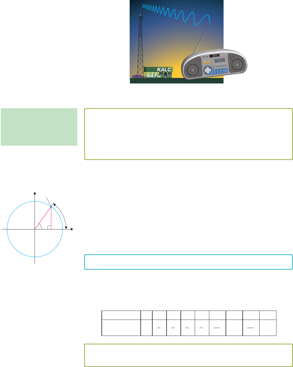
Manyphenomena encountered in your daily life involve waves. For instance, music is trans-
mittedfromradiostations inthe formofelectromagneticwaves.Yourradioreceiverdecodes
these electromagnetic waves and causes a thin membrane inside the speakers to vibrate,
which, in turn, creates pressure waves in the air. When these waves reach your ears, you
hear the music from your radio. (See Figure 0.41.) Each of these waves is periodic, meaning
P1: OSO/OVY P2: OSO/OVY QC: OSO/OVY T1: OSO
MHDQ256-Ch00 MHDQ256-Smith-v1.cls December 8, 2010 15:25
LT (Late Transcendental)
CONFIRMING PAGES
28 CHAPTER 0
..
Preliminaries 0-28
that the basic shape of the wave is repeated over and over again. The mathematical descrip-
tion of such phenomena involves periodic functions, the most familiar of which are the
trigonometric functions. First, we remind you of a basic definition.
FIGURE 0.41
Radio and sound waves
DEFINITION 4.1
A function f is periodic of period T if
f (x + T ) = f (x)
for all x such that x and x + T are in the domain of f. The smallest such number
T > 0 is called the fundamental period.
NOTES
When we discuss the period of a
function, we most often focus on
the fundamental period.
There are several equivalent ways of defining the sine and cosine functions. We want
to emphasize a simple definition from which you can easily reproduce many of the basic
properties of these functions. Referring to Figure 0.42, begin by drawing the unit circle
x
2
+ y
2
= 1. Let θ be the angle measured (counterclockwise) from the positive x-axis to
the line segment connecting the origin to the point (x, y) on the circle. Here, we measure θ
in radians, given by the length of the arc indicated in the figure. Again referring to Figure
0.42, we define sin θ to be the y-coordinate of the point on the circle and cos θ to be the
x-coordinate of the point.From this definition, it follows that sin θ and cos θ are defined for
all values of θ, so that each has domain −∞ <θ<∞, while the range for each of these
functions is the interval [−1, 1].
y
x
u
u
(cos u, sin u)
sin u
cos u
1
FIGURE 0.42
Definition of sin θ and cos θ :
cos θ = x and sin θ = y
REMARK 4.1
Unless otherwise noted, we always measure angles in radians.
Note that since the circumference of a circle (C = 2πr) of radius 1 is 2π , we have that
360
◦
corresponds to 2π radians. Similarly, 180
◦
corresponds to π radians, 90
◦
corresponds
to π/2 radians and so on. In the accompanying table, we list some common angles as
measured in degrees, together with the corresponding radian measures.
Angle in degrees 0
◦
30
◦
45
◦
60
◦
90
◦
135
◦
180
◦
270
◦
360
◦
Angle in radians 0
π
6
π
4
π
3
π
2
3π
4
π
3π
2
2π
THEOREM 4.1
The functions f (θ) = sinθ and g(θ) = cos θ are periodic, of period 2π.
P1: OSO/OVY P2: OSO/OVY QC: OSO/OVY T1: OSO
MHDQ256-Ch00 MHDQ256-Smith-v1.cls December 8, 2010 15:25
LT (Late Transcendental)
CONFIRMING PAGES
0-29 SECTION 0.4
..
Trigonometric Functions 29
PROOF
Referring to Figure 0.42, since a complete circle is 2π radians, adding 2π to any angle takes
you all the way around the circle and back to the same point (x, y). This says that
sin(θ +2π) = sin θ
and
cos(θ +2π) = cos θ,
for all values of θ. Furthermore, 2π is the smallest positive angle for which this is true.
Youarelikelyalreadyfamiliarwith thegraphsof f (x) = sin x and g(x) = cos x shown
in Figures 0.43a and 0.43b, respectively.
y
1
1
q wwrr q
x
y
1
1
p 2p2p p
x
FIGURE 0.43a
y = sin x
FIGURE 0.43b
y = cos x
x sin x cos x
0 0 1
π
6
1
2
√
3
2
π
4
√
2
2
√
2
2
π
3
√
3
2
1
2
π
2
1 0
2π
3
√
3
2
−
1
2
3π
4
√
2
2
−
√
2
2
5π
6
1
2
−
√
3
2
π 0 −1
3π
2
−1 0
2π 0 1
Notice that you could slide the graph of y = sin x slightly to the left or right and get an
exact copy of the graph of y = cos x. Specifically, we have the relationship
sin
x +
π
2
= cos x.
The accompanying table lists some common values of sine and cosine. Notice that
many of these can be read directly from Figure 0.42.
EXAMPLE 4.1 Solving Equations Involving Sines and Cosines
Find all solutions of the equations (a) 2 sin x − 1 = 0 and (b) cos
2
x −3cos x + 2 = 0.
Solution For (a), notice that 2sin x − 1 = 0if2sinx = 1orsinx =
1
2
. From the unit
circle, we find that sin x =
1
2
if x =
π
6
or x =
5π
6
. Since sin x has period 2π , additional
solutions are
π
6
+ 2π,
5π
6
+ 2π,
π
6
+ 4π and so on. A convenient way of indicating that
any integer multiple of 2π can be added to either solution is to write x =
π
6
+ 2nπ or
x =
5π
6
+ 2nπ, for any integer n. Part (b) may look rather difficult at first. However,
notice that it looks like a quadratic equation using cos x instead of x. With this clue, you
can factor the left-hand side to get
0 = cos
2
x −3cos x + 2 = (cos x −1)(cos x −2),
from which it follows that either cos x = 1orcosx = 2. Since −1 ≤ cos x ≤ 1 for all
x, the equation cos x = 2 has no solution. However, we get cos x = 1ifx = 0, 2π or
any integer multiple of 2π. We can summarize all the solutions by writing x = 2nπ , for
any integer n.
REMARK 4.2
Instead of writing (sin θ)
2
or
(cos θ)
2
, we usually use the
notation sin
2
θ and cos
2
θ,
respectively. Further, we often
suppress parentheses and write,
for example, sin2x, instead of
sin(2x).
We now give definitions of the remaining four trigonometric functions.
P1: OSO/OVY P2: OSO/OVY QC: OSO/OVY T1: OSO
MHDQ256-Ch00 MHDQ256-Smith-v1.cls December 8, 2010 15:25
LT (Late Transcendental)
CONFIRMING PAGES
30 CHAPTER 0
..
Preliminaries 0-30
DEFINITION 4.2
The tangent function is defined by tan x =
sin x
cos x
.
The cotangent function is defined by cot x =
cos x
sin x
.
The secant function is defined by sec x =
1
cos x
.
The cosecant function is defined by csc x =
1
sin x
.
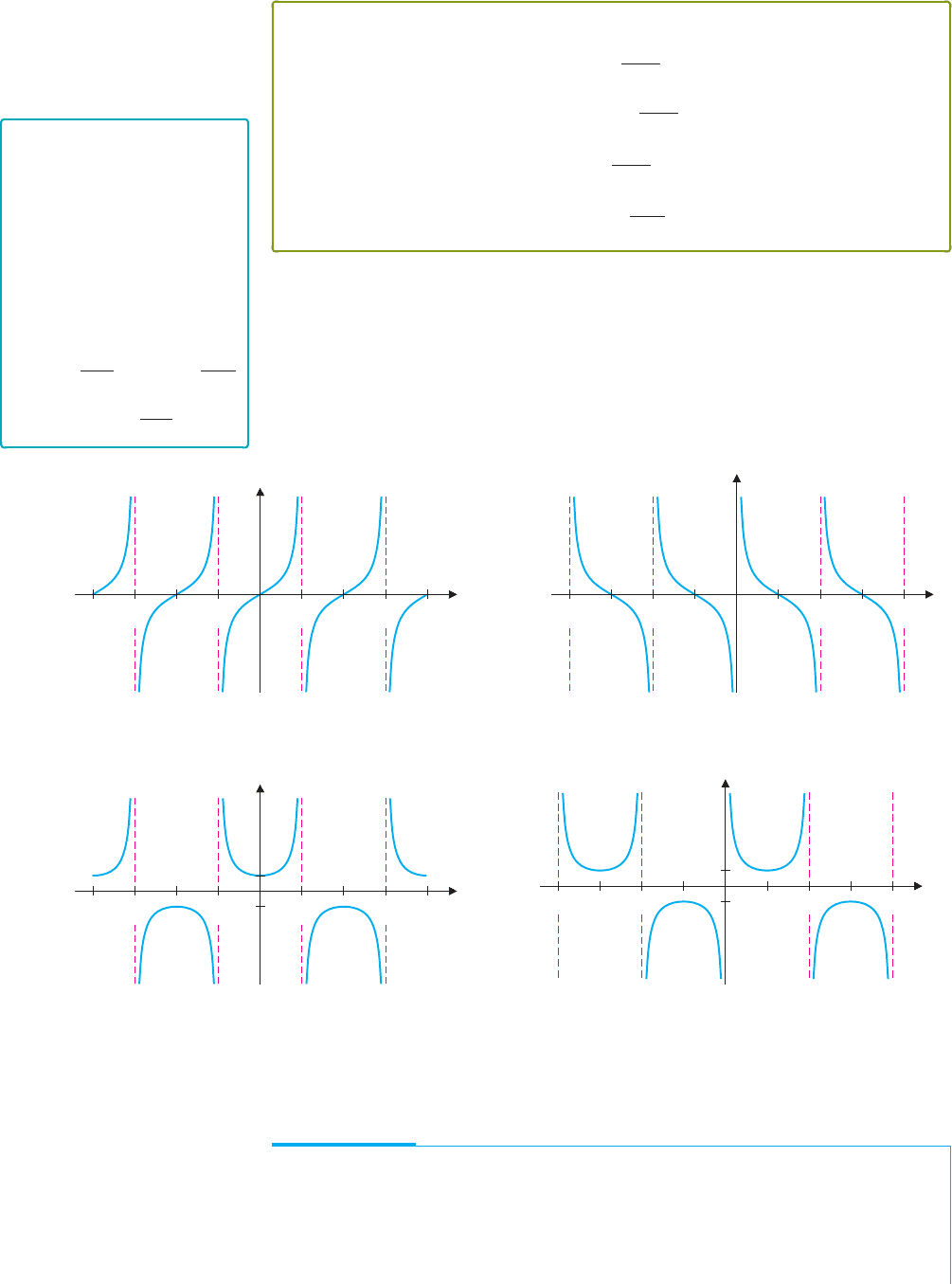
We show graphs of these functions in Figures 0.44a–0.44d. Notice in each graph the loca-
tions of the vertical asymptotes. For the “co” functions cot x and csc x, the division by sin x
causes vertical asymptotes at 0, ±π, ±2π and so on (where sin x = 0). For tan x and sec x,
the division by cos x produces vertical asymptotes at ±π/2, ±3π/2, ±5π/2 and so on
(where cosx = 0). Once you have determined the vertical asymptotes, the graphs are rela-
tively easy to draw.
REMARK 4.3
Most calculators have keys for
the functions sin x, cos x and
tan x, but not for the other three
trigonometric functions. This
reflects the central role that
sin x, cos x and tan x play in
applications. To calculate
function values for the other
three trigonometric functions,
you can simply use the identities
cot x =
1
tan x
, sec x =
1
cos x
and csc x =
1
sin x
.
Notice that tan x and cot x are periodic, of period π , while sec x and csc x are periodic,
of period 2π.
p
2p
2p
p
w
w
qq
y
x
p
2p
2p
p
w
w
qq
y
x
FIGURE 0.44a
y = tan x
FIGURE 0.44b
y = cot x
p
2p
2p
p
w
w
qq
y
x
1
1
p 2p
2p
p
w
w
q
q
y
x
1
1
FIGURE 0.44c
y = sec x
FIGURE 0.44d
y = csc x
It is important to learn the effect of slight modifications of these functions. We present
a few ideas here and in the exercises.
EXAMPLE 4.2 Altering Amplitude and Period
Graph y = 2 sin x and y = sin2x, and describe how each differs from the graph of
y = sin x. (See Figure 0.45a.)
Solution The graph of y = 2 sin x is given in Figure 0.45b. Notice that this graph is
similar to the graph of y = sin x, except that the y-values oscillate between −2 and 2,
P1: OSO/OVY P2: OSO/OVY QC: OSO/OVY T1: OSO
MHDQ256-Ch00 MHDQ256-Smith-v1.cls December 8, 2010 15:25
LT (Late Transcendental)
CONFIRMING PAGES
0-31 SECTION 0.4
..
Trigonometric Functions 31
w
w
q
q
y
x
2
1
1
2
w
w
q
q
y
x
2
1
1
2
y
x
2
1
1
2
p2pp2p
FIGURE 0.45a
y = sin x
FIGURE 0.45b
y = 2 sin x
FIGURE 0.45c
y = sin (2x)
instead of −1 and 1. Next, the graph of y = sin2x is given in Figure 0.45c. In this case,
the graph is similar to the graph of y = sin x, except that the period is π instead of 2π
(so that the oscillations occur twice as fast).
The results in example 4.2 can be generalized. For A > 0, the graph of y = A sin x
oscillates between y =−A and y = A. In this case, we call A the amplitude of the sine
curve. Notice that for any positive constant c, the period of y = sin cx is 2π/c. Similarly,
for the function A cos cx, the amplitude is A and the period is 2π/c.
The sine and cosine functions can be used to model sound waves. A pure tone (think of
a tuning fork note) is a pressure wave described by the sinusoidal function A sin ct. (Here,
we are using the variable t, since the air pressure is a function of time.) The amplitude A
determines how loud the tone is perceived to be and the period determines the pitch of the
note. In this setting, it is convenient to talk about the frequency f = c/2π . The higher
the frequency is, the higher the pitch of the note will be. (Frequency is measured in hertz,
where 1 hertz equals 1 cycle per second.) Note that the frequency is simply the reciprocal
of the period.
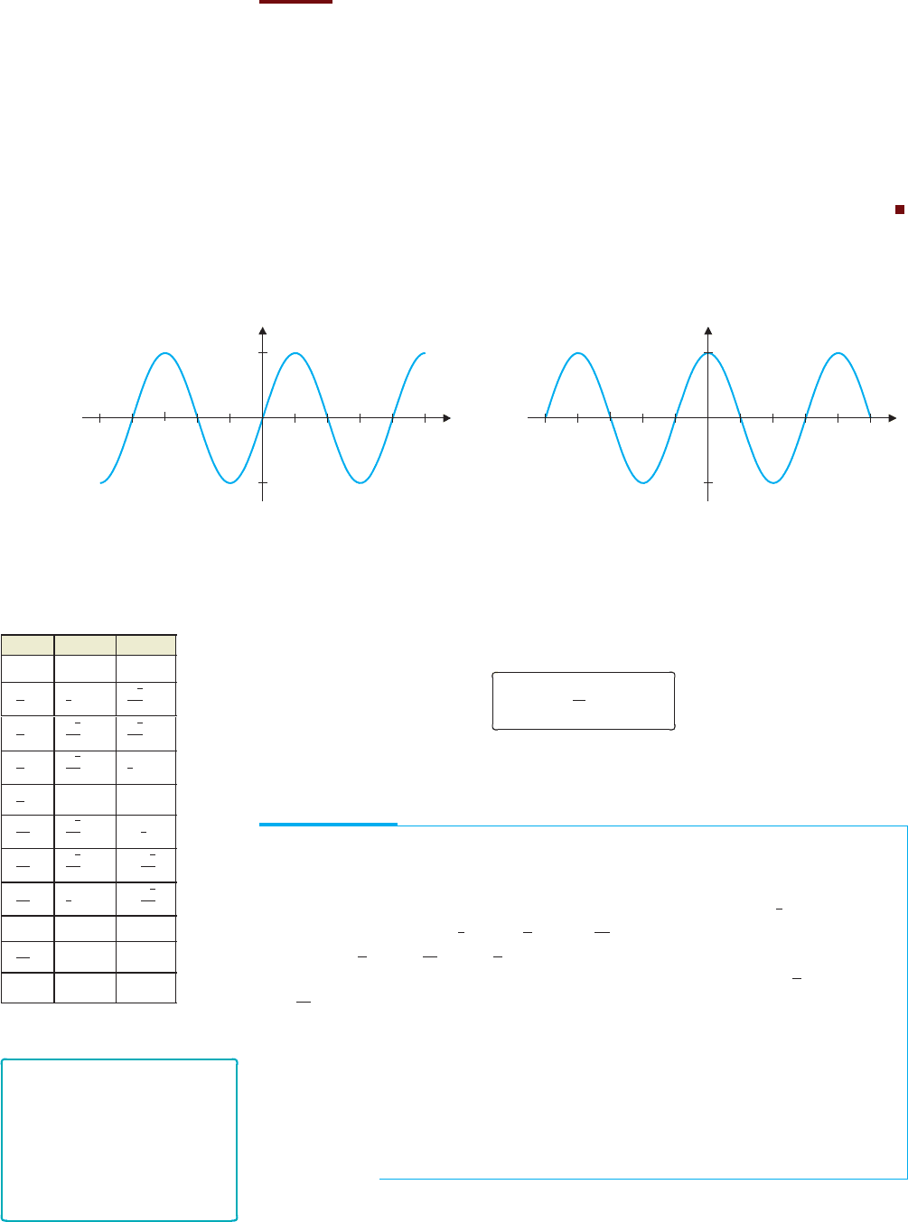
EXAMPLE 4.3 Finding Amplitude, Period and Frequency
Find the amplitude, period and frequency of (a) f (x) = 4cos 3x and
(b) g(x) = 2sin(x/3).
Solution (a) For f (x), the amplitude is 4, the period is 2π/3 and the frequency
is 3/(2π). (See Figure 0.46a.) (b) For g(x), the amplitude is 2, the period is
2π/(1/3) = 6π and the frequency is 1/(6π). (See Figure 0.46b.)
y
2p2p
4
4
i o
i
o
x
y
x
2p 3pp2p3p p
2
2
FIGURE 0.46a
y = 4 cos 3x
FIGURE 0.46b
y = 2 sin (x/3)

P1: OSO/OVY P2: OSO/OVY QC: OSO/OVY T1: OSO
MHDQ256-Ch00 MHDQ256-Smith-v1.cls December 8, 2010 15:25
LT (Late Transcendental)
CONFIRMING PAGES
32 CHAPTER 0
..
Preliminaries 0-32
There are numerous formulas or identities that are helpful in manipulating the trigono-
metric functions. You should observe that, from the definition of sin θ and cos θ (see
Figure 0.42), the Pythagorean Theorem gives us the familiar identity
sin
2
θ +cos
2
θ = 1,
since the hypotenuse of the indicated triangle is 1. This is true for any angle θ . In addition,
sin(−θ) =−sinθ and cos(−θ) = cosθ.
We list several important identities in Theorem 4.2.
THEOREM 4.2
For any real numbers α and β, the following identities hold:
sin(α + β) = sin α cos β + sinβ cosα (4.1)
cos(α + β) = cos α cos β − sinα sin β (4.2)
sin
2
α =
1
2
(1 − cos2α) (4.3)
cos
2
α =
1
2
(1 + cos2α).
(4.4)
From the basic identitiessummarized in Theorem 4.2, numerousother useful identities
can be derived. We derive two of these in example 4.4.
EXAMPLE 4.4 Deriving New Trigonometric Identities
Derive the identities sin2θ = 2sinθ cosθ and cos 2θ = cos
2
θ −sin
2
θ.
Solution These can be obtained from formulas (4.1) and (4.2), respectively, by
substituting α = θ and β = θ. Alternatively, the identity for cos2θ can be obtained by
subtracting equation (4.3) from equation (4.4).
Two kinds of combinations of sine and cosine functions are especially important in
applications.In thefirst type, a sine andcosine with the same period butdifferentamplitudes
are added.
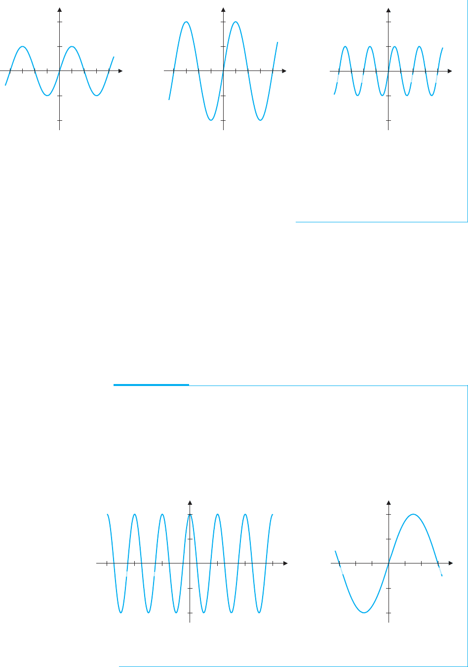
EXAMPLE 4.5 Combinations of Sines and Cosines
Graph f (x) = 3cos x + 4sin x and describe the resulting graph.
Solution You should get something like the graph in Figure 0.47. Notice that the
graph looks very much like a sine curve with period 2π and amplitude 5, but it has been
shifted about 0.75 unit to the left. Alternatively, you could say that it looks like a cosine
curve, shifted about 1 unit to the right. Using the appropriate identity, you can verify
these guesses.
y
4
x
3p⫺3pp2p⫺2p ⫺p
⫺4
FIGURE 0.47
y = 3 cos x + 4 sin x