Smith R., Minton R. Calculus

Подождите немного. Документ загружается.

P1: OSO/OVY P2: OSO/OVY QC: OSO/OVY T1: OSO

MHDQ256-Ch13 MHDQ256-Smith-v1.cls December 31, 2010 16:55

LT (Late Transcendental)

CONFIRMING PAGES

13-35 SECTION 13.3

Partial Derivatives 843

50. Given the contour plot of f below, what can be said about

(0, 0)? f

(0, 0)?

In exercises 51–54, ﬁnd a function with the given

properties.

51. f

= 2x sin y + 3x

, f

= x

cos y + 2x

y +

√

52. f

= ye

+ 1

, f

= xe

+ y cos y

53. f

+ y

− 1

, f

+ 1

+ y

54. f



y/x + 2 cos(2x + y), f



x/y + cos (2x + y)

APPLICATIONS

55. (a) Showthatthefunctions f

(x, t) = sinnπ x cos nπct satisfy

the wave equation c

∂

∂x

∂

∂t

, for any positive integer

n and any constant c.

(b) Show that if f (x) is a function with a continuous second

derivative, then f (x −ct) and f (x + ct) are both solutions

of the wave equation. If x represents position and t repre-

sents time, explain why c can be interpreted as the velocity

of the wave.

56. (a) The value of an investment of $1000 invested at a constant

10% rate for 5 years is V = 1000



1 + 0.1(1 − T )

1 + I



where T is the tax rate and I is the inﬂation rate. Com-

pute

∂V

∂ I

and

∂V

∂T

, and discuss whether the tax rate or the

inﬂation rate has a greater inﬂuence on the value of the

investment.

(b) The value of an investment of $1000 invested at a rate r for

5 years with a tax rate of 28% is V = 1000



1 + 0.72r

1 + I



where I is the inﬂation rate. Compute

∂V

∂r

and

∂V

∂ I

and discuss whether the investment rate or the inﬂa-

tion rate has a greater inﬂuence on the value of the

investment.

57. Supposethattheposition of a guitarstringoflengthL variesac-

cordingto p(x, t) = sin x cost,wherex representsthe distance

along the string, 0 ≤ x ≤ L, and t represents time. Compute

and interpret

∂p

∂x

and

∂p

∂t

58. Suppose that the concentration of some pollutant in a

river as a function of position x and time t is given by

p(x, t) = p

(x − ct)e

−μt

for constants p

, c and μ. Show that

∂p

∂t

=−c

∂p

∂x

− μp. Interpret both

∂p

∂t

and

∂p

∂x

, and explain

how this equation relates the change in pollution at a speciﬁc

location to the current of the river and the rate at which the

pollutant decays.

59. (a) In a chemical reaction, the temperature T, entropy S, Gibbs

free energy G and enthalpyH are related by G = H − TS.

Show that

∂(G/T )

∂T

=−

(b) Show that

∂(G/T )

∂(1/T )

= H. Chemists measure the enthalpy

of a reaction by measuring this rate of change.

60. Suppose that three resistors are in parallel in an electri-

cal circuit. If the resistances are R

, R

and R

ohms,

respectively, then the net resistance in the circuit equals

R =

+ R

.Compute andinterpretthepartial

derivative

∂ R

. Given this partial derivative, explain how to

quickly write down the partial derivatives

∂ R

and

∂ R

61. A process called tag-and-recapture is used to estimate pop-

ulations of animals in the wild. First, some number T of

the animals are captured, tagged and released into the wild.

Later, a number S of the animals are captured, of which t

are observed to be tagged. The estimate of the total pop-

ulation is then P(T, S, t) =

. Compute P(100, 60, 15);

the proportion of tagged animals in the recapture is

Based on your estimate of the total population, what propor-

tion of the total population has been tagged? Now compute

∂ P

∂t

(100, 60, 15) and use it to estimate howmuchyour popula-

tionestimatewouldchangeifonemorerecaptured animalwere

tagged.

62. Let T (x, y) be the temperature at longitude x and latitude y in

the United States. In general, explain why you would expect

to have

∂T

∂y

< 0. If a cold front is moving from east to west,

would you expect

∂T

∂x

to be positive or negative?

63. Suppose that L hours of labor and K dollars of investment

by a company result in a productivity of P = L

0.75

0.25

(a) Compute the marginal productivity of labor, deﬁned

∂ P

∂ L

and the marginal productivity of capital, deﬁned

∂ P

∂ K

. (b) Show that

∂

∂ L

< 0 and

∂

∂ K

< 0. Interpret this

in terms of diminishing returns on investments in labor and

capital. (c) Show that

∂

∂ L∂ K

> 0 and interpret it in economic

terms.

64. Suppose that the demand for coffee is given by

= 300 +

− 5p

and the demand for sugar is given by

= 250 +

− 6p

, where p

is the price of a pound of

coffee and p

is the price of a pound of sugar. Show that

∂ D

∂p

P1: OSO/OVY P2: OSO/OVY QC: OSO/OVY T1: OSO

MHDQ256-Ch13 MHDQ256-Smith-v1.cls December 31, 2010 16:55

LT (Late Transcendental)

CONFIRMING PAGES

844 CHAPTER 13

Functions of Several Variables and Partial Differentiation 13-36

and

∂ D

∂p

are both negative. This is the deﬁnition of comple-

mentary commodities. Interpret the partial derivatives and

explain why the word complementary is appropriate.

65. Suppose that D

, p

) and D

, p

) are demand

functions for commodities coffee and tea with prices p

and p

, respectively. If

∂ D

∂p

and

∂ D

∂p

are both posi-

tive, explain why the commodities are called substitute

commodities.

EXPLORATORY EXERCISES

1. In exercises 47 and 48, you interpreted the second-order

partial derivatives f

and f

in terms of concavity. In

this exercise, you will develop a geometric interpretation

of the mixed partial derivative f

. (More information can

be found in the article “What is f

?” by Brian Mc-

Cartin in the March 1998 issue of the journal PRIMUS.)

Start by using Taylor’s Theorem (see section 9.7) to show

that

lim

k→0

lim

h→0

f (x, y) − f (x + h, y) − f (x, y + k)

+ f (x + h, y + k)

= f

(x, y).

[Hint: Treating y as a constant, you have f (x + h, y) =

f (x, y) +hf

(x, y) + h

g(x, y), for some function g(x, y).

Similarly, expand the other terms in the numerator.] There-

fore, for small h and k, f

(x, y) ≈

− f

+ f

where f

= f (x, y), f

= f (x +h, y), f

= f (x, y +k) and

= f (x +h, y +k). The four points P

= (x, y, f

), P

(x + h, y, f

), P

= (x, y + k, f

) and P

= (x +h, y +

k, f

) determine a parallelepiped, as shown in the ﬁgure.

Recalling that the volume of a parallelepiped formed by vec-

tors a, b and c is givenby |a ·(b ×c)|, show that the volume of

this box equals |( f

− f

+ f

)hk|. That is, the volume

is approximately equal to | f

(x, y)|(hk)

. Conclude that the

larger | f

(x, y)| is, the greater the volume of the box and

hence, the farther the point P

is from the plane determined by

the points P

, P

and P

. To see what this means graphically,

start with the function f (x, y) = x

+ y

at the point (1, 1, 2).

With h = k = 0.1, show that the points (1, 1, 2), (1.1, 1,

2.21), (1, 1.1, 2.21) and (1.1, 1.1, 2.42) all lie in the same

plane. The derivative f

(1, 1) = 0 indicates that at the point

(1.1, 1.1, 2.42), the graph does not curve away from the plane

of the points (1, 1, 2), (1.1, 1, 2.21) and (1, 1.1, 2.21). Contrast

this to the behavior of the function f (x, y) = x

+ xy at the

point (1, 1, 2). This says that f

measures the amount of

curving of the surface as you sequentially change x and y by

small amounts.

2. For a function g(x, y), deﬁne F(x) =



g(x, y)dy. In this

exercise, you will explore the question of whether or not



(x) =



∂g

∂x

(x, y)dy. (a) Show that this is true for

g(x, y) = e

. (b) Show that it is true for g(x, y) = h(x)k(y)

if k is continuous andh is differentiable. (c) Show that it istrue

for g(x, y) =

on the interval [0, 2]. (d) Find numerically

that it is not true for g(x, y) =

. (e) Conjecture condi-

tions on the function g(x, y) for which the statement is true.

(f) A mathematician would say that the underlying issue in

this problem is the interchangeability of limits and integrals.

Explain how limits are involved.

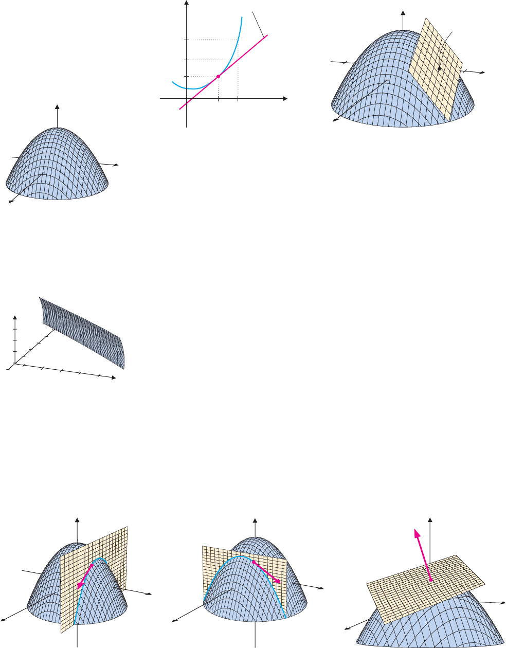
13.4 TANGENT PLANES AND LINEAR APPROXIMATIONS

Recall that the tangent line to the curve y = f (x)atx = a stays close to the curve near the

point of tangency, enabling us to use the tangent line to approximate values of the function

close to the point of tangency. (See Figure 13.24a.) The equation of the tangent line is

given by

y = f (a) + f



(a)(x −a). (4.1)

In section 3.1, we called this the linear approximation to f (x)atx = a.

In much the same way, we can approximate the value of a function of two variables

near a given point using the tangent plane to the surfaceat that point. Forinstance, the graph

of z = 6 − x

− y

and its tangent plane at the point (1, 2, 1) are shown in Figure 13.24b.

Notice that near the point (1, 2, 1), the surface and the tangent plane are very close together.

Refer to Figures 13.25a and 13.25b to visualize the process. Starting from a standard

graphingwindow(Figure13.25ashowsz = 6− x

− y

with−3 ≤ x ≤ 3and−3 ≤ y ≤ 3),

P1: OSO/OVY P2: OSO/OVY QC: OSO/OVY T1: OSO

MHDQ256-Ch13 MHDQ256-Smith-v1.cls December 31, 2010 16:55

LT (Late Transcendental)

CONFIRMING PAGES

13-37 SECTION 13.4

Tangent Planes and Linear Approximations 845

a x

f(x

)

f(a)

y  f(x)

y  f(a)  f(a)(x  a)

(1, 2.1)

FIGURE 13.24a FIGURE 13.24b

Linear approximation z = 6 − x

− y

and the

tangent plane at (1, 2, 1)

zoom in on the point (1, 2, 1), as in Figure 13.25b (showing z = 6 − x

− y

with

0.9 ≤ x ≤ 1.1 and 1.9 ≤ y ≤ 2.1). The surface in Figure 13.25b looks like a plane, since

we have zoomed in sufﬁciently far that the surface and its tangent plane are difﬁcult to

distinguish visually. This suggests that for points (x, y) close to the point of tangency, we

can use the corresponding z-value on the tangent plane as an approximation to the value

of the function at that point. We begin by looking for an equation of the tangent plane to

z = f (x, y) at the point (a, b, f (a, b)), where f

and f

are continuous at (a, b). For this,

FIGURE 13.25a

z = 6 − x

− y

, with −3 ≤ x ≤ 3

and −3 ≤ y ≤ 3

FIGURE 13.25b

z = 6 − x

− y

, with

0.9 ≤ x ≤ 1.1 and 1.9 ≤ y ≤ 2.1

we need only ﬁnd a vector normal to the plane, since one point lying in the tangent plane

is the point of tangency (a, b, f (a, b)). To ﬁnd a normal vector, we will ﬁnd two vectors

lying in the plane and then take their cross product to obtain a vector orthogonal to both

(and thus, orthogonal to the plane).

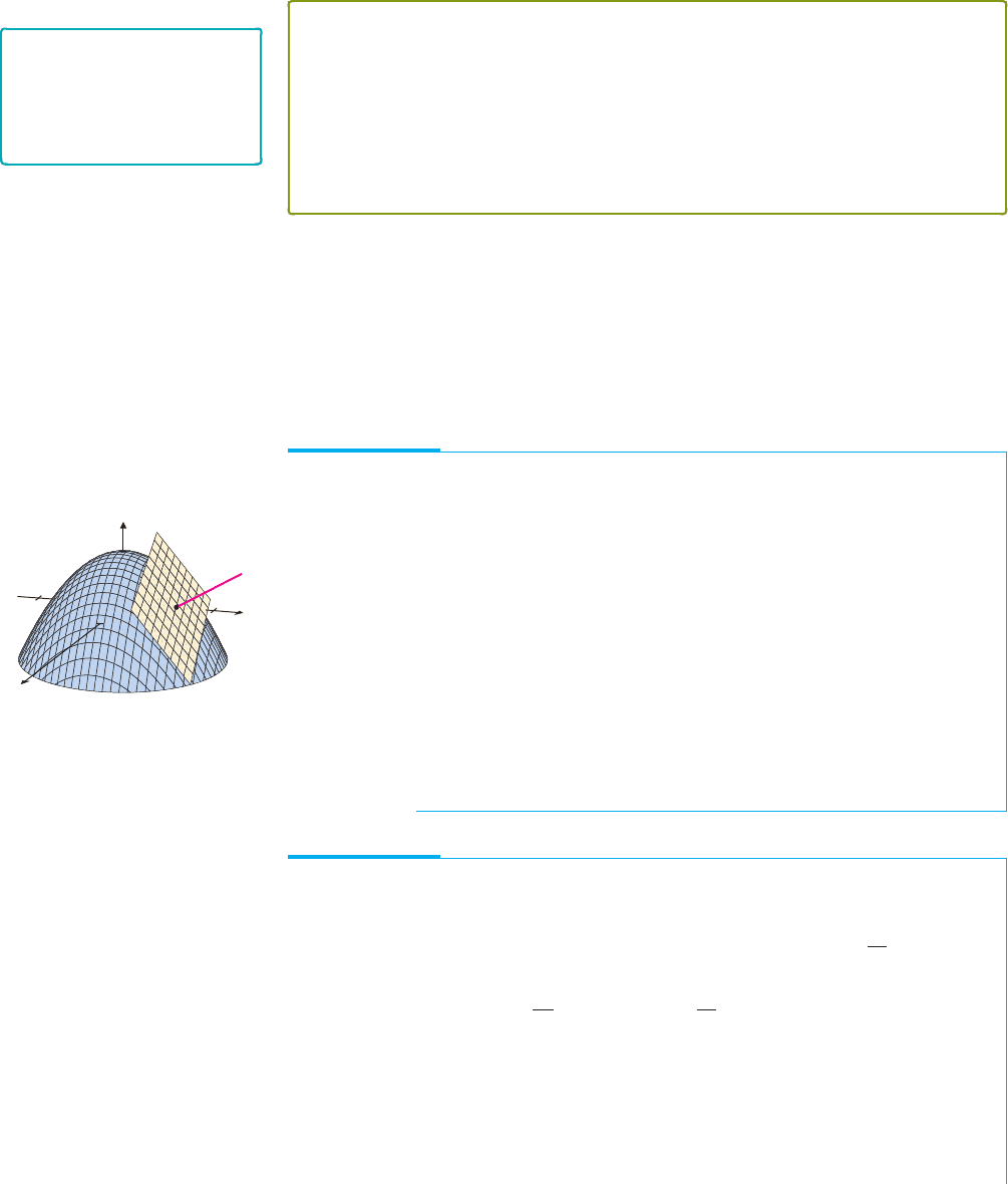
Imagine intersecting the surface z = f (x, y) with the plane y = b, as shown in Figure

13.26a. As we observed in section 13.3, the result is a curve in the plane y = b whose

slope at x = a is given by f

(a, b). Along the tangent line at x = a, a change of 1 unit in

x corresponds to a change of f

(a, b)inz. Since we’re looking at a curve that lies in the

plane y = b, the value of y doesn’t change at all along the curve. A vector with the same

direction as the tangent line is then 1, 0, f

(a, b). This vector must then be parallel to

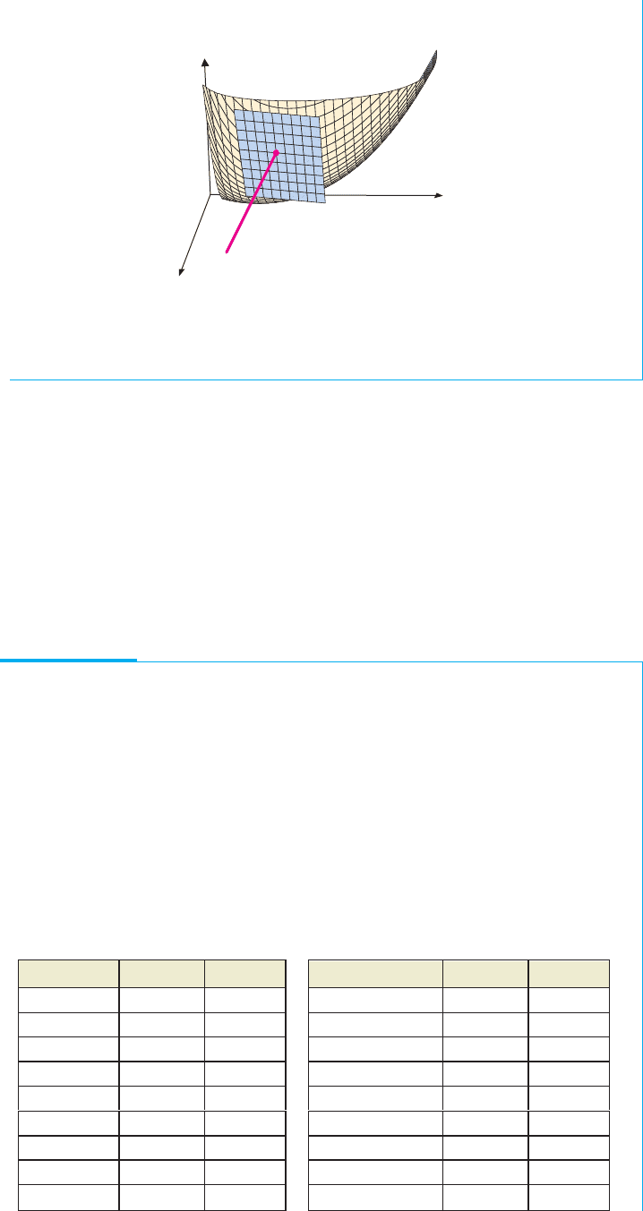
the tangent plane. (Think about this some.) Similarly, intersecting the surface z = f (x, y)

with the plane x = a, as shown in Figure 13.26b, we get a curve lying in the plane x = a,

whose slope at y = b is given by f

(a, b). A vector with the same direction as the tangent

line at y = b is then 0, 1, f

(a, b).

FIGURE 13.26a

The intersection of the surface

z = f (x, y) with the plane y = b

FIGURE 13.26b

The intersection of the surface

z = f (x, y) with the plane x = a

FIGURE 13.26c

Tangent plane and normal vector

P1: OSO/OVY P2: OSO/OVY QC: OSO/OVY T1: OSO

MHDQ256-Ch13 MHDQ256-Smith-v1.cls December 31, 2010 16:55

LT (Late Transcendental)

CONFIRMING PAGES

846 CHAPTER 13

Functions of Several Variables and Partial Differentiation 13-38

We have now found two vectors that are parallel to the tangent plane: 1, 0, f

(a, b)

and 0, 1, f

(a, b). A vector normal to the plane is then given by the cross product:

0, 1, f

(a, b)×1, 0, f

(a, b)=f

(a, b), f

(a, b), −1.

We indicate the tangent plane and normal vector at a point in Figure 13.26c (on the pre-

ceeding page). We have the following result.

REMARK 4.1

Notice the similarity between

the equation of the tangent

plane given in (4.2) and the

equation of the tangent line to

y = f (x) given in (4.1).

THEOREM 4.1

Suppose that f (x, y) has continuous ﬁrst partial derivatives at (a, b). A normal vector

to the tangent plane to z = f (x, y)at(a, b) is then  f

(a, b), f

(a, b), −1. Further,

an equation of the tangent plane is given by

z − f (a, b) = f

(a, b)(x − a) + f

(a, b)(y − b)

or z = f (a, b) + f

(a, b)(x − a) + f

(a, b)(y − b). (4.2)

Observe that since we now know a normal vector to the tangent plane, the line orthogonal

to the tangent plane and passing through the point (a, b, f (a, b)) is given by

x = a + f

(a, b)t, y = b + f

(a, b)t, z = f (a, b) − t. (4.3)

This line is called the normal line to the surface at the point (a, b, f (a, b)).

It’s now a simple matter to use Theorem 4.1 to construct the equations of a tangent

plane and normal line to nearly any surface, as we illustrate in examples 4.1 and 4.2.

EXAMPLE 4.1 Finding Equations of the Tangent Plane

and the Normal Line

Find equations of the tangent plane and the normal line to z = 6 − x

− y

at the point

(1, 2, 1).

Solution For f (x, y) = 6 − x

− y

,wehave f

=−2x and f

=−2y. This gives

us f

(1, 2) =−2 and f

(1, 2) =−4. A normal vector is then −2, −4, −1 and from

(4.2), an equation of the tangent plane is

z = 1 − 2(x − 1) − 4(y − 2).

From (4.3), equations of the normal line are

x = 1 −2t, y = 2 −4t, z = 1 −t.

A sketch of the surface, the tangent plane and the normal line is shown in

Figure 13.27.



FIGURE 13.27

Surface, tangent plane and normal

line at the point (1, 2, 1)

EXAMPLE 4.2 Finding Equations of the Tangent Plane

and the Normal Line

Find equations of the tangent plane and the normal line to z = x

+ y

at (2, 1, 13).

Solution Here, f

= 3x

and f

= 3y

−

, so that f

(2, 1) = 12 +4 = 16

and f

(2, 1) = 3 −4 =−1. A normal vector is then 16, −1, −1 and from (4.2), an

equation of the tangent plane is

z = 13 + 16(x − 2) − (y − 1).

From (4.3), equations of the normal line are

x = 2 +16t, y = 1 −t, z = 13 −t.

P1: OSO/OVY P2: OSO/OVY QC: OSO/OVY T1: OSO

MHDQ256-Ch13 MHDQ256-Smith-v1.cls December 31, 2010 16:55

LT (Late Transcendental)

CONFIRMING PAGES

13-39 SECTION 13.4

Tangent Planes and Linear Approximations 847

A sketch of the surface, the tangent plane and the normal line is shown in Figure 13.28.

FIGURE 13.28

Surface, tangent plane and normal line

at the point (2, 1, 13)



In Figures 13.27 and 13.28, the tangent plane appears to stay close to the surface near

the point of tangency. This says that for (x, y) close to the point of tangency, the z-values

on the tangent plane should be close to the corresponding z-values on the surface, which

are given by the function values f (x, y). Further, the simple form of the equation for the

tangent plane makes it ideal for approximating the value of complicated functions.

We deﬁne the linear approximation L(x, y)of f (x, y) at the point (a, b)tobethe

function deﬁning the z-values on the tangent plane, namely,

L(x, y) = f (a, b) + f

(a, b)(x − a) + f

(a, b)(y − b), (4.4)

from (4.2). We illustrate this with example 4.3.

EXAMPLE 4.3 Finding a Linear Approximation

Compute the linear approximation of f (x, y) = 2x +e

−y

at (0, 0). Compare the linear

approximation to the actual function values for (a) x = 0 and y near 0; (b) y = 0 and x

near 0; (c) y = x, with both x and y near 0 and (d) y = 2x, with both x and y near 0.

Solution Here, f

= 2 + 2xe

−y

and f

=−e

−y

, so that f

(0, 0) = 2 and

(0, 0) =−1. Also, f (0, 0) = 1. From (4.4), the linear approximation is then given by

L(x, y) = 1 +2(x −0) −(y − 0) = 1 + 2x − y.

The following table compares values of L(x, y) and f (x, y) for a number of points of

the form (0, y), (x, 0), (x, x) and (x, 2x).

(x, y) f (x, y) L(x, y)

(0, 0.1) 0.905 0.9

(0, 0.01) 0.99005 0.99

(0, −0.1) 1.105 1.1

(0, −0.01) 1.01005 1.01

(0.1, 0) 1.21005 1.2

(0.01, 0) 1.02010 1.02

(−0.1, 0) 0.81005 0.8

(−0.01, 0) 0.98010 0.98

(x, y) f (x, y) L(x, y)

(0.1, 0.1) 1.11393 1.1

(0.01, 0.01) 1.01015 1.01

(−0.1, −0.1) 0.91628 0.9

(−0.01, −0.01) 0.99015 0.99

(0.1, 0.2) 1.02696 1.0

(0.01, 0.02) 1.00030 1.0

(−0.1, −0.2) 1.03368 1.0

(−0.01, −0.02) 1.00030 1.0

P1: OSO/OVY P2: OSO/OVY QC: OSO/OVY T1: OSO

MHDQ256-Ch13 MHDQ256-Smith-v1.cls December 31, 2010 16:55

LT (Late Transcendental)

CONFIRMING PAGES

848 CHAPTER 13

Functions of Several Variables and Partial Differentiation 13-40

Notice that the closer a given point is to the point of tangency, the more accurate the

linear approximation tends to be at that point. This is typical of this type of

approximation. We will explore this further in the exercises.



f(a  x)

f(a)

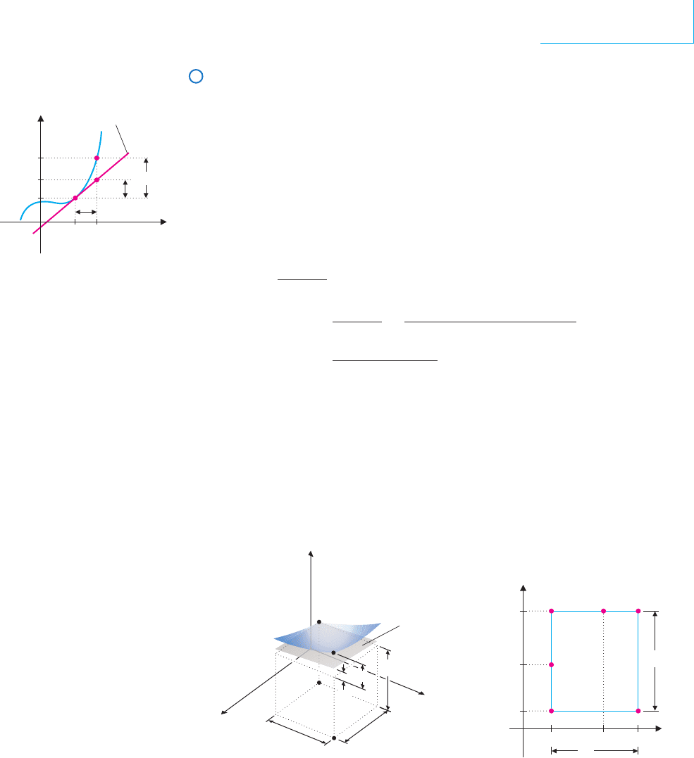
y  f(x)

y  f(a)  f(a)(x  a)

aa  x

x

y

FIGURE 13.29

Increments and differentials for a

function of one variable

Increments and Differentials

Now that we have examined linear approximations from a graphical perspective, we will

examine them in a symbolic fashion. First, we remind you of the notation and some alter-

native language that we used in section 3.1 for functions of a single variable. We deﬁned

the increment y of the function f (x)atx = a to be

y = f (a +x) − f (a).

Referring to Figure 13.29, notice that for x small,

y ≈ dy = f



(a)x,

where we referred to dy as the differential of y. Further, observe that if f is differentiable at

x = a and ε =

y − dy

x

, then we have

ε =

y − dy

x

f (a + x) − f (a) − f



(a)x

x

f (a + x) − f (a)

x

− f



(a) → 0,

as x → 0. (You’ll need to recognize the deﬁnition of derivative here!) Finally, solving for

y in terms of ε,wehave

y = dy + ε x,

where ε → 0, as x → 0. We can make a similar observation for functions of several

variables, as follows.

For z = f (x, y), we deﬁne the increment of f at (a, b)tobe

z = f (a + x, b +y) − f (a, b).

x

y

Tangen

plane

(a, b, 0)

z  f(x, y)

(a, b, f (a, b))

(a   x, b  y, 0)

f(a, b)

z

a  x

(u, b  y)

(a, v)

b  y

y

x

FIGURE 13.30 FIGURE 13.31

Linear approximation Intermediate points from the

Mean Value Theorem

That is, z is the change in z that occurs when a is incremented by x and b is incre-

mented by y, as illustrated in Figure 13.30. Notice that as long as f is continuous in

some open region containing (a, b) and f has ﬁrst partial derivatives on that region, we

can write

z = f (a + x, b +y) − f (a, b)

= [ f (a + x, b +y) − f (a, b + y)] + [ f (a, b + y) − f (a, b)]

Adding and subtracting f (a, b + y).

P1: OSO/OVY P2: OSO/OVY QC: OSO/OVY T1: OSO

MHDQ256-Ch13 MHDQ256-Smith-v1.cls December 31, 2010 16:55

LT (Late Transcendental)

CONFIRMING PAGES

13-41 SECTION 13.4

Tangent Planes and Linear Approximations 849

= f

(u, b + y)[(a + x) − a] + f

(a,v)[(b +y) −b]

Applying the Mean Value Theorem to both terms.

= f

(u, b + y)x + f

(a,v)y,

by the Mean Value Theorem. Here, u is some value between a and a + x, and v is some

value between b and b + y. (See Figure 13.31.) This gives us

z = f

(u, b + y)x + f

(a,v)y

={f

(a, b) +[ f

(u, b + y) − f

(a, b)]}x

+{f

(a, b) +[ f

(a,v) − f

(a, b)]}y,

which we rewrite as

z = f

(a, b)x + f

(a, b)y + ε

x + ε

y,

where ε

= f

(u, b + y) − f

(a, b) and ε

= f

(a,v) − f

(a, b).

Finally, observethat if f

and f

are both continuous in some open region containing (a, b),

then ε

and ε

will both tend to 0, as (x, y) → (0, 0). In fact, you should recognize that

since ε

,ε

→ 0, as (x, y) → (0, 0), the products ε

x and ε

y both tend to 0 even

faster than do ε

,ε

, x or y individually. (Think about this!)

We have now established the following result.

THEOREM 4.2

Suppose that z = f (x, y) is deﬁned on the rectangular region

R ={(x, y)|x

< x < x

, y

< y < y

} and f

and f

are deﬁned on R and are

continuous at (a, b) ∈ R. Then for (a +x, b +y) ∈ R,

z = f

(a, b)x + f

(a, b)y + ε

x + ε

y, (4.5)

where ε

and ε

are functions of x and y that both tend to zero, as

(x, y) → (0, 0).

For some very simple functions, we can compute z by hand, as illustrated in

example 4.4.

EXAMPLE 4.4 Computing the Increment z

For z = f (x, y) = x

− 5xy, ﬁnd z and write it in the form indicated in Theorem 4.2.

Solution We have

z = f (x + x, y + y) − f (x, y)

= [(x + x)

− 5(x + x)(y + y)] − (x

− 5xy)

= x

+ 2x x + (x)

− 5(xy + x y + y x + x y) − x

+ 5xy

= (2x − 5y)



 

x + (−5x)



 

y + (x)





x + (−5x)



 

y

= f

(x, y) x + f

(x, y) y + ε

x + ε

y,

where ε

= x and ε

=−5x both tend to zero, as (x, y) → (0, 0), as indicated in

Theorem 4.2. You should observe here that by grouping the terms differently, we could

get different choices for ε

and ε



Look closely at the ﬁrst two terms in the expansion of the increment z given in (4.5).

If we take x = x − a and y = y − b, then they correspond to the linear approximation

of f (x, y). In this context, we give this a special name. If we increment x by the amount

P1: OSO/OVY P2: OSO/OVY QC: OSO/OVY T1: OSO

MHDQ256-Ch13 MHDQ256-Smith-v1.cls December 31, 2010 16:55

LT (Late Transcendental)

CONFIRMING PAGES

850 CHAPTER 13

Functions of Several Variables and Partial Differentiation 13-42

dx = x and increment y by dy = y, then we deﬁne the differential of z to be

dz = f

(x, y) dx + f

(x, y) dy.

This is sometimes referred to as a total differential. Notice that for dx and dy small, we

have from (4.5) that

z ≈ dz.

You should recognize that this is the same approximation as the linear approximation

developed in the beginning of this section. In this case, though, we have developed this

from an analytical perspective, rather than the geometrical one used in the beginning of the

section.

In Deﬁnition 4.1, we givea special name to functions that can be approximated linearly

in the above fashion.

DEFINITION 4.1

Let z = f (x, y). We say that f is differentiable at (a, b) if we can write

z = f

(a, b)x + f

(a, b)y + ε

x + ε

y,

where ε

and ε

are both functions of x and y and ε

,ε

→ 0, as

(x, y) → (0, 0). We say that f is differentiable on a region R ⊂ R

whenever f is

differentiable at every point in R.

Although this deﬁnition of a differentiable function may not appear to be an obvious

generalization of the corresponding deﬁnition for a function of a single variable, in fact, it

is. We explore this in exercises 49 and 50.

Notethat from Theorem4.2, if f

and f

aredeﬁned on someopen rectangle R contain-

ing the point (a, b) and if f

and f

are continuous at (a, b), then f will be differentiable at

(a, b). Just as withfunctions ofa single variable, it can be shownthat if f is differentiableat a

point (a, b), then it is also continuous at (a, b). Further, owing to Theorem 4.2, if a function

is differentiableat a point, then the linear approximation(differential) at that point provides

a good approximation to the function near that point. Be very careful of what this does not

say, however. If a function has partial derivatives at a point, it need not be differentiable or

even continuous at that point. (In exercises 35 and 36, you will see examples of a function

with partial derivatives deﬁned everywhere, but that is not differentiable at a point.)

The idea of a linear approximation extends easily to three or more dimensions. We lose

the graphical interpretation of a tangent plane approximating a surface, but the deﬁnition

should make sense.

DEFINITION 4.2

The linear approximation to f (x, y, z) at the point (a, b, c)isgivenby

L(x, y, z) = f (a, b, c) + f

(a, b, c)(x − a)

+ f

(a, b, c)(y − b) + f

(a, b, c)(z − c).

We can writethe linear approximation in the context of incrementsand differentials, as

follows.Ifweincrementx byx, y byy andz byz,thentheincrementofw = f (x, y, z)

is given by

w = f (x +x, y + y, z + z) − f (x, y, z)

≈ dw = f

(x, y, z)x + f

(x, y, z)y + f

(x, y, z)z.

P1: OSO/OVY P2: OSO/OVY QC: OSO/OVY T1: OSO

MHDQ256-Ch13 MHDQ256-Smith-v1.cls December 31, 2010 16:55

LT (Late Transcendental)

CONFIRMING PAGES

13-43 SECTION 13.4

Tangent Planes and Linear Approximations 851

A good way to interpret (and remember!) the linear approximation is that each partial

derivative represents the change in the function relative to the change in that variable. The

linear approximation starts with the function value at the known point and adds in the

approximate changes corresponding to each of the independent variables.

EXAMPLE 4.5 Approximating the Sag in a Beam

Suppose that the sag in a beam of length L, width w and height h is given by

S(L,w,h) = 0.0004

, with all lengths measured in inches. We illustrate the beam

in Figure 13.32. A beam is supposed to measure L = 36,w = 2 and h = 6 with a

corresponding sag of 1.5552 inches. Due to weathering and other factors, the

manufacturer only guarantees measurements with error tolerances L = 36 ±1,

w = 2 ±0.4 and h = 6 ±0.8. Use a linear approximation to estimate the possible

range of sags in the beam.

Solution We ﬁrst compute

∂ S

∂ L

= 0.0016

∂ S

∂w

=−0.0004

and

∂ S

∂h

=−0.0012

. At the point (36, 2, 6), we then have

∂ S

∂ L

(36, 2, 6) = 0.1728,

∂ S

∂w

(36, 2, 6) =−0.7776 and

∂ S

∂h

(36, 2, 6) =−0.7776. From Deﬁnition 4.2, the linear

approximation of the sag is then given by

S ≈ 1.5552 + 0.1728(L −36) −0.7776(w − 2) − 0.7776(h − 6).

Notice that we could have written this in differential form using Deﬁnition 4.1.

From the stated tolerances, L − 36 must be between −1 and 1, w −2 must be

between −0.4 and 0.4 and h − 6 must be between −0.8 and 0.8. Notice that the

maximum sag then occurs with L − 36 = 1,w−2 =−0.4 and h − 6 =−0.8. The

linear approximation predicts that

S − 1.5552 ≈ 0.1728 +0.31104 +0.62208 = 1.10592.

Similarly, the minimum sag occurs with L − 36 =−1,w−2 = 0.4 and h −6 = 0.8.

The linear approximation predicts that

S − 1.5552 ≈−0.1728 − 0.31104 − 0.62208 =−1.10592.

Based on the linear approximation, the sag is 1.5552 ± 1.10592, or between

0.44928 and 2.66112. As you can see, in this case, the uncertainty in the sag is

substantial.



FIGURE 13.32

A typical beam

In many real-world situations, we do not have a formula for the quantity we are inter-

ested in computing. Even so, given sufﬁcient information, we can still use linear approxi-

mations to estimate the desired quantity.

EXAMPLE 4.6 Estimating the Gauge of a Sheet of Metal

Manufacturing plants create rolls of metal of a desired gauge (thickness) by feeding the

metal through very large rollers. The thickness of the resulting metal depends on the

gap between the working rollers, the speed at which the rollers turn and the temperature

of the metal. Suppose that for a certain metal, a gauge of 4 mm is produced by a gap of

4 mm, a speed of 10 m/s and a temperature of 900

◦

. Experiments show that an increase

in speed of 0.2 m/s increases the gauge by 0.06 mm and an increase in temperature of

◦

decreases the gauge by 0.04 mm. Use a linear approximation to estimate the gauge

at 10.1 m/s and 880

◦

Solution With no change in gap, we assume that the gauge is a function g(s, t)

of the speed s and the temperature t. Based on our data,

∂g

∂s

≈

0.06

0.2

= 0.3 and

P1: OSO/OVY P2: OSO/OVY QC: OSO/OVY T1: OSO

MHDQ256-Ch13 MHDQ256-Smith-v1.cls December 31, 2010 16:55

LT (Late Transcendental)

CONFIRMING PAGES

852 CHAPTER 13

Functions of Several Variables and Partial Differentiation 13-44

∂g

∂t

≈

−0.04

=−0.004. From Deﬁnition 4.2, the linear approximation of g(s, t)

is given by

g(s, t) ≈ 4 +0.3(s − 10) − 0.004(t − 900).

With s = 10.1 and t = 880, we get the estimate

g(10.1, 880) ≈ 4 +0.3(0.1) −0.004(−20) = 4.11.



BEYOND FORMULAS

You should think of linear approximations more in terms of example 4.6 than example

4.5. That is, linear approximations are most commonly used when there is no known

formula for the function f. You can then read equation (4.4) or Deﬁnition 4.2 as a

recipe that tells you which ingredients (i.e., function values and derivatives) you need

toapproximatea function value.The visualimagebehind this formula, showninFigure

13.30, gives you information about how good your approximation is.

EXERCISES 13.4

WRITING EXERCISES

1. Describewhich graphical properties ofthe surface z = f (x, y)

would cause the linear approximation of f at (a, b) to be par-

ticularly accurate or inaccurate.

2. Temperature varieswith longitude (x), latitude (y) and altitude

(z). Speculate whether or not the temperature function would

be differentiable and what signiﬁcance the answer would have

for weather prediction.

3. Imagine a surface z = f (x, y) with a ridge of discontinuities

along the line y = x. Explain in graphical terms why f would

not be differentiable at (0, 0) or any other point on the line

y = x.

4. The function in exercise 3 might have ﬁrst partial derivatives

(0, 0) and f

(0, 0). Explain why the slopes along x = 0 and

y = 0 could have limits as x and y approach 0. If differentiable

is intended to describe functions with smooth graphs, explain

why differentiability is not deﬁned in terms of the existence of

partial derivatives.

In exercises 1–6, ﬁnd equations of the tangent plane and normal

line to the surface at the given point.

1. z = x

+ y

− 1 at (a) (2, 1, 4) and (b) (0, 2, 3)

2. z = e

−x

−y

at (a) (0, 0, 1) and (b) (1, 1, e

−2

)

3. z = sin x cos y at (a) (0,π,0) and (b) (

,π,−1)

4. z = x

− 2xy at (a) (−2, 3, 4) and (b) (1, −1, 3)

5. z =



+ y

at (a) (−3, 4, 5) and (b) (8, −6, 10)

6. z =

at (a) (1, 2, 2) and (b) (−1, 4, −1)

............................................................

In exercises7–12, compute the linear approximation of the func-

tion at the given point.

7. f (x, y) =



+ y

at (a) (3, 0) and (b) (0, −3)

8. f (x, y) = sin x cos y at (a)





and (b)





9. f (x, y, z) = sin

−1

x + tan (yz) at (a)



0,π,



and

(b)



√

, 2, 0



10. f (x, y, z) = xe

−



x − y

at (a) (4, 1, 0) and (b) (1, 0, 2)

11. f (w, x, y, z) = w

xy −e

wyz

at (a) (−2, 3, 1, 0) and

(b) (0, 1, −1, 2)

12. f (w, x, y, z) = cos xyz − w

at (a) (2, −1, 4, 0) and

(b) (2, 1, 0, 1)

............................................................

In exercises 13–16, compare the linear approximation from the

indicated exercise to the exact function value at the given points.

13. Exercise 7 part (a) at (3, −0.1), (3.1, 0), (3.1, −0.1)

14. Exercise 7 part (b) at (0.1, −3), (0, −3.1), (0.1, −3.1)

15. Exercise 9 part (a) at (0, 3,

), (0.1, π,

), (0, π, 0.2)

16. Exercise 9 part (b) at (0.7, 2, 0), (0.7, 1.9, 0), (0.7, 2, 0.1)

............................................................

17. Use a linear approximation to estimate the range of sags

in the beam of example 4.5 if the error tolerances are

L = 36 ±0.5,w = 2 ±0.2 and h = 6 ±0.5.

18. Use a linear approximation to estimate the range of sags

in the beam of example 4.5 if the error tolerances are

L = 32 ±0.4,w = 2 ±0.3 and h = 8 ±0.4.