Smith R., Minton R. Calculus
Подождите немного. Документ загружается.

P1: OSO/OVY P2: OSO/OVY QC: OSO/OVY T1: OSO
MHDQ256-Ch13 MHDQ256-Smith-v1.cls December 31, 2010 16:55
LT (Late Transcendental)
CONFIRMING PAGES
13-25 SECTION 13.3
..
Partial Derivatives 833
60. (a) Showthatthefunction f (x, y) =
⎧
⎨
⎩
xy
2
x
2
+ y
4
, if(x, y) = (0, 0)
0, if(x, y) = (0,0)
is not continuous at (0, 0). Notice that this function
is closely related to that of example 2.5. (b) Show
that this function “acts” continuous in the sense that
lim
(x,y)→(0,0)
y=kx
f (x, y) = f (0, 0) for any k.
61. Suppose that several level curves of a function f meet
at (a, b). Does lim
(x,y)→(a,b)
f (x, y) exist? Is f continuous
at (a, b)?
62. If f and g arecontinuous at (a, b), prove that f + g and f − g
are continuous at (a, b).
............................................................
In exercises 63–66, use polar coordinates to find the indicated
limit, if it exists. Note that (x, y) → (0, 0) is equivalent to r → 0.
63. lim
(x,y)→(0,0)
x
2
+ y
2
sin
x
2
+ y
2
64. lim
(x,y)→(0,0)
e
x
2
+y
2
− 1
x
2
+ y
2
65. lim
(x,y)→(0,0)
xy
2
x
2
+ y
2
66. lim
(x,y)→(0,0)
x
2
y
x
2
+ y
2
EXPLORATORY EXERCISES
1. In this exercise, you will explore how the patterns of contour
plots relate to the existence of limits. Start by showing that
lim
(x,y)→(0,0)
x
2
x
2
+ y
2
doesn’t exist and lim
(x,y)→(0,0)
x
2
y
x
2
+ y
2
= 0.
Then sketch several contour plots for each function while
zooming in on the point (0, 0). For a function whose limit
exists as (x, y) approaches (a, b), what should be happening to
the range of function valuesas you zoom in on the point (a, b)?
Describe the appearance of each contour plot for
x
2
y
x
2
+ y
2
near
(0, 0). By contrast, what should be happening to the range of
function values as you zoom in on a point at which the limit
doesn’t exist? Explain howthis appears inthe contour plots for
x
2
x
2
+ y
2
. Use contour plots to conjecture whether or not the
following limits exist: lim
(x,y)→(0,0)
xy
x
2
+ y
and lim
(x,y)→(0,0)
x sin y
x
2
+ y
2
.
2. Find a function g(y) such that f (x, y) is continuous for
f (x, y) =
(1 + xy)
1/x
, if x = 0
g(y), if x = 0
.
13.3 PARTIAL DERIVATIVES
In this section, we generalize the notion of derivative to functions of more than one variable.
First, recall that for a function f of a single variable, we define the derivative function as
f
(x) = lim
h→0
f (x +h) − f (x)
h
,
for any values of x for which the limit exists. At any particular value x = a, we interpret
f
(a) as the instantaneous rate of change of the function with respect to x at that point.
a a h
(a, b)
(a h, b)
b
h
R
y
x
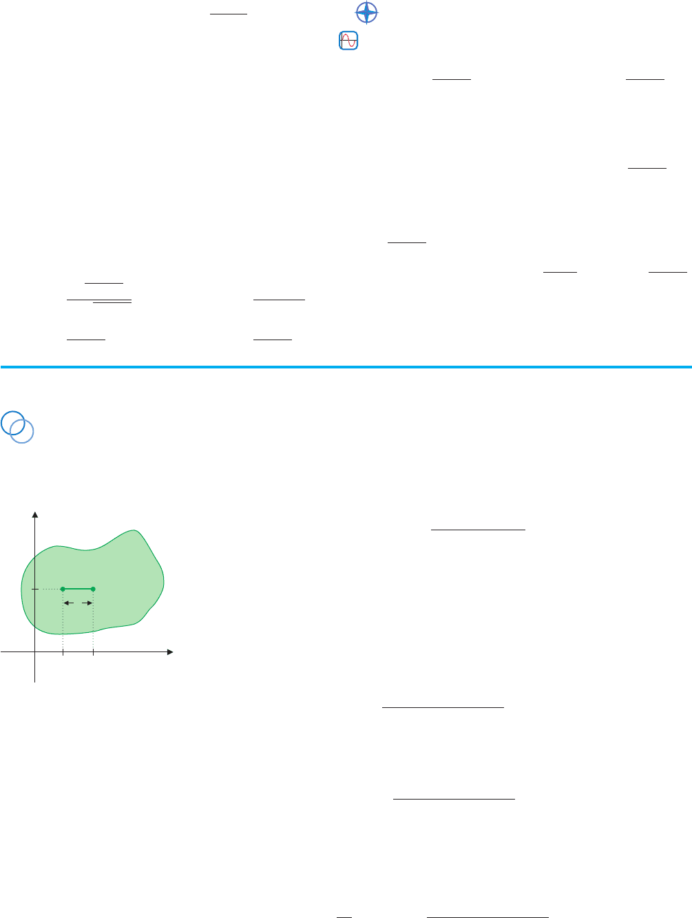
FIGURE 13.19
Average temperature on a horizontal
line segment
Consider a flat metal plate in the shape of the region R ⊂ R
2
, where the temperature
at any point (x, y) ∈ R is given by f (x, y). If you move along the horizontal line segment
from (a, b)to(a + h, b) (as in Figure 13.19), notice that y is a constant (y = b). So, the
average rate of change of the temperature with respect to the horizontal distance x on this
line segment is given by
f (a + h, b) − f (a, b)
h
.
To get the instantaneous rate of change of f in the x-direction at the point (a, b), we take
the limit as h → 0:
lim
h→0
f (a + h, b) − f (a, b)
h
.
You should recognize this limit as a derivative. Since f is a function of two variables and
we have held the one variable fixed (y = b), we call this the partial derivative of f with
respect to x at the point (a, b), denoted
∂ f
∂x
(a, b) = lim
h→0
f (a + h, b) − f (a, b)
h
.
P1: OSO/OVY P2: OSO/OVY QC: OSO/OVY T1: OSO
MHDQ256-Ch13 MHDQ256-Smith-v1.cls December 31, 2010 16:55
LT (Late Transcendental)
CONFIRMING PAGES
834 CHAPTER 13
..
Functions of Several Variables and Partial Differentiation 13-26
z
y
x
z
a
x
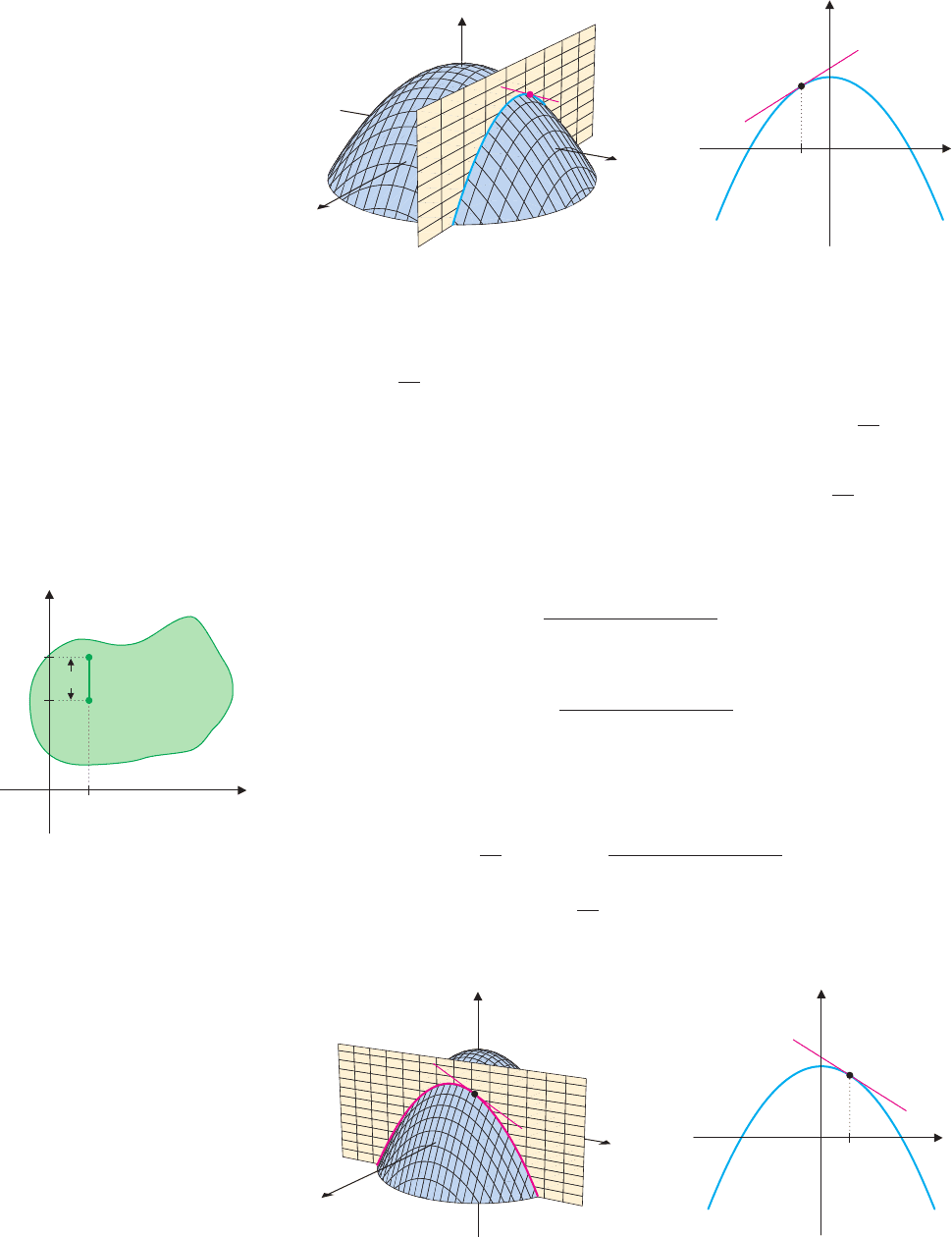
FIGURE 13.20a FIGURE 13.20b
Intersection of the surface The curve z = f (x, b)
z = f (x, y) with the plane y = b
This says that
∂ f
∂x
(a, b) gives the instantaneous rate of change of f with respect to x (i.e.,
in the x-direction) at the point (a, b). Graphically, observe that in defining
∂ f
∂x
(a, b), we are
looking only at points in the plane y = b. The intersection of z = f (x, y) and y = b is a
curve, as shown in Figures 13.20a and 13.20b. The partial derivative
∂ f
∂x
(a, b) then gives
the slope of the tangent line to this curve at x = a, as indicated in Figure 13.20b.
a
(a, b)
(a, b h)
b
h
R
y
x
b h
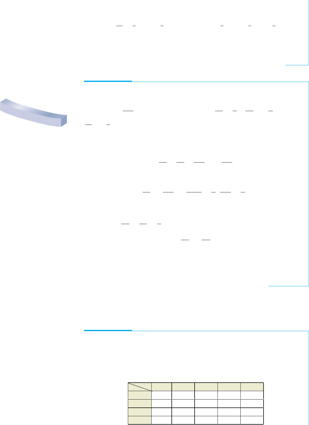
FIGURE 13.21
Average temperature on a vertical
line segment
Alternatively, if we move along a vertical line segment from (a, b)to(a, b + h) (as in
Figure 13.21), the average rate of change of f along this segment is given by
f (a, b + h) − f (a, b)
h
.
The instantaneous rate of change of f in the y-direction at the point (a, b) is then given by
lim
h→0
f (a, b + h) − f (a, b)
h
,
which you should again recognize as a derivative. In this case, however, we have held the
value of x fixed (x = a) and refer to this as the partial derivative of f with respect to y at
the point (a, b), denoted
∂ f
∂y
(a, b) = lim
h→0
f (a, b + h) − f (a, b)
h
.
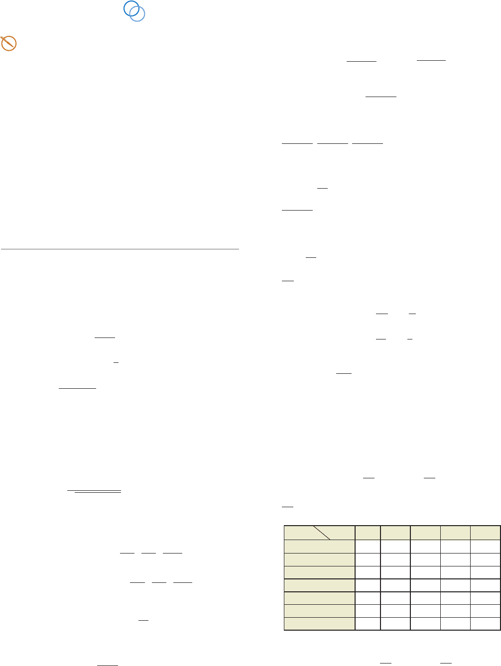
Graphically, observe that in defining
∂ f
∂y
(a, b), we are looking only at points in the plane
x = a. The intersection of z = f (x, y) and x = a is a curve, as shown in Figures 13.22a
z
y
x
z
b
y
FIGURE 13.22a FIGURE 13.22b
The intersection of the surface The curve z = f (a, y)
z = f (x, y) with the plane x = a

P1: OSO/OVY P2: OSO/OVY QC: OSO/OVY T1: OSO
MHDQ256-Ch13 MHDQ256-Smith-v1.cls December 31, 2010 16:55
LT (Late Transcendental)
CONFIRMING PAGES
13-27 SECTION 13.3
..
Partial Derivatives 835
and 13.22b. In this case, notice that the partial derivative
∂ f
∂y
(a, b) gives the slope of the
tangent line to the curve at y = b, as shown in Figure 13.22b.
More generally, we define the partial derivative functions as follows.
DEFINITION 3.1
The partial derivative of f (x, y) with respect to x, written
∂ f
∂x
, is defined by
∂ f
∂x
(x, y) = lim
h→0
f (x +h, y) − f (x, y)
h
,
for any values of x and y for which the limit exists.
The partial derivative of f (x, y) with respect to y, written
∂ f
∂y
, is defined by
∂ f
∂y
(x, y) = lim
h→0
f (x, y + h) − f (x, y)
h
,
for any values of x and y for which the limit exists.
With functions of several variables, we can no longer use the prime notation for denoting
partial derivatives. [Which partial derivative would f
(x, y) denote?] So, we introduce
several convenient types of notation here. For z = f (x, y), we write
∂ f
∂x
(x, y) = f
x
(x, y) =
∂z
∂x
(x, y) =
∂
∂x
[ f (x, y)].
Theexpression
∂
∂x
isapartial differential operator. Ittellsyoutotakethepartialderivative
(with respect to x) of whatever expression follows it. Similarly, we have
∂ f
∂y
(x, y) = f
y
(x, y) =
∂z
∂y
(x, y) =
∂
∂y
[ f (x, y)].
Fortunately, we can compute partial derivatives using all of our usual rules for com-
puting ordinary derivatives, as follows. Notice that in the definition of
∂ f
∂x
, the value of y is
held constant, say at y = b. If we define g(x) = f (x, b), then
∂ f
∂x
(x, b) = lim
h→0
f (x +h, b) − f (x, b)
h
= lim
h→0
g(x + h) − g(x)
h
= g
(x).
That is, to compute the partial derivative
∂ f
∂x
, you simply take an ordinary derivative with
respect to x, while treating y as a constant. Similarly, you can compute
∂ f
∂y
by taking an
ordinary derivative with respect to y, while treating x as a constant.
EXAMPLE 3.1 Computing Partial Derivatives
For f (x, y) = 3x
2
+ x
3
y + 4y
2
, compute
∂ f
∂x
(x, y),
∂ f
∂y
(x, y), f
x
(1, 0) and f
y
(2, −1).
Solution Compute
∂ f
∂x
by treating y as a constant. We have
∂ f
∂x
=
∂
∂x
(3x
2
+ x
3
y + 4y
2
) = 6x + (3x
2
)y + 0 = 6x + 3x
2
y,

P1: OSO/OVY P2: OSO/OVY QC: OSO/OVY T1: OSO
MHDQ256-Ch13 MHDQ256-Smith-v1.cls December 31, 2010 16:55
LT (Late Transcendental)
CONFIRMING PAGES
836 CHAPTER 13
..
Functions of Several Variables and Partial Differentiation 13-28
where the partial derivative of 4y
2
with respect to x is 0, since 4y
2
is treated as if it were
a constant when differentiating with respect to x. Next, we compute
∂ f
∂y
by treating x as
a constant. We have
∂ f
∂y
=
∂
∂y
(3x
2
+ x
3
y + 4y
2
) = 0 + x
3
(1) + 8y = x
3
+ 8y.
Substituting values for x and y,weget
f
x
(1, 0) =
∂ f
∂x
(1, 0) = 6 +0 = 6
and
f
y
(2, −1) =
∂ f
∂y
(2, −1) = 8 −8 = 0.
Since we are holding one of the variables fixed when we compute a partial derivative,
we have the product rules:
∂
∂x
(uv) =
∂u
∂x
v + u
∂v
∂x
and
∂
∂y
(uv) =
∂u
∂y
v + u
∂v
∂y
and the quotient rule:
∂
∂x
u
v
=
∂u
∂x
v − u
∂v
∂x
v
2
,
with a corresponding quotient rule holding for
∂
∂y
u
v
.
EXAMPLE 3.2 Computing Partial Derivatives
For f (x, y) = e
xy
+
x
y
, compute
∂ f
∂x
and
∂ f
∂y
.
Solution Treating y as a constant, we have from the chain rule that
∂ f
∂x
=
∂
∂x
e
xy
+
x
y
= ye
xy
+
1
y
.
Similarly, treating x as a constant, we have
∂ f
∂y
=
∂
∂y
e
xy
+
x
y
= xe
xy
−
x
y
2
.
We interpret partial derivatives as rates of change, in the same way as we interpret
ordinary derivatives of functions of a single variable.
EXAMPLE 3.3 An Application of Partial Derivatives
to Thermodynamics
For a real gas, van der Waals’ equation states that
P +
n
2
a
V
2
(V − nb) = nRT,

P1: OSO/OVY P2: OSO/OVY QC: OSO/OVY T1: OSO
MHDQ256-Ch13 MHDQ256-Smith-v1.cls December 31, 2010 16:55
LT (Late Transcendental)
CONFIRMING PAGES
13-29 SECTION 13.3
..
Partial Derivatives 837
where P is the pressure of the gas, V is the volume of the gas, T is the temperature (in
degrees Kelvin), n is the number of moles of gas, R is the universal gas constant and a
and b are constants. Compute and interpret
∂ P(V, T )
∂V
and
∂T(P,V )
∂ P
.
Solution We first solve for P to get
P =
nRT
V −nb
−
n
2
a
V
2
and compute
∂ P(V ,T )
∂V
=
∂
∂V
nRT
V −nb
−
n
2
a
V
2
=−
nRT
(V − nb)
2
+ 2
n
2
a
V
3
.
TODAY IN
MATHEMATICS
Shing-Tung Yau (1949– )
A Chinese-born mathematician
who earned a Fields Medal for
his contributions to algebraic
geometry and partial differential
equations. A strong supporter of
mathematics education in China,
he established the Institute of
Mathematical Science in Hong
Kong, the Morningside Center of
Mathematics of the Chinese
Academy of Sciences and the
Center of Mathematical Sciences
at Zhejiang University. His work
has been described by colleagues
as “extremely deep and
powerful” and as showing
“enormous technical power and
insight. He has cracked problems
on which progress has been
stopped for years.”
Notice that this gives the rate of change of pressure relative to a change in volume (with
temperature held constant). Next, solving van der Waals’ equation for T,weget
T =
1
nR
P +
n
2
a
V
2
(V − nb)
and compute
∂T(P,V )
∂ P
=
∂
∂ P
1
nR
P +
n
2
a
V
2
(V − nb)
=
1
nR
(V − nb).
This givesthe rate of change of temperature relative to a change in pressure (with volume
held constant). In exercise 20, you will have an opportunity to discover an interesting
fact about these partial derivatives.
Noticethat the partial derivativesfound inthe preceding examples are themselvesfunc-
tions of two variables. We have seen that second- and higher-order derivatives of functions
of a single variable provide much significant information. Not surprisingly, higher-order
partial derivatives are also very important in applications.
For functions of two variables, there are four different second-order partial deriva-
tives. The partial derivative with respect to x of
∂ f
∂x
is
∂
∂x
∂ f
∂x
, usually abbreviated as
∂
2
f
∂x
2
or f
xx
. Similarly, taking two successive partial derivatives with respect to y gives us
∂
∂y
∂ f
∂y
=
∂
2
f
∂y
2
= f
yy
. For mixed second-order partial derivatives, one derivative is
taken with respect to each variable. If the first partial derivative is taken with respect to x,
we have
∂
∂y
∂ f
∂x
, abbreviated as
∂
2
f
∂y∂x
, or ( f
x
)
y
= f
xy
. If the first partial derivative is
taken with respect to y,wehave
∂
∂x
∂ f
∂y
, abbreviated as
∂
2
f
∂x∂y
,or(f
y
)
x
= f
yx
.
EXAMPLE 3.4 Computing Second-Order Partial Derivatives
Find all second-order partial derivatives of f (x, y) = x
2
y − y
3
+ ln x.
Solution We start by computing the first-order partial derivatives:
∂ f
∂x
= 2xy +
1
x
and
∂ f
∂y
= x
2
− 3y
2
. We then have
∂
2
f
∂x
2
=
∂
∂x
∂ f
∂x
=
∂
∂x
2xy +
1
x
= 2y −
1
x
2
,
∂
2
f
∂y∂x
=
∂
∂y
∂ f
∂x
=
∂
∂y
2xy +
1
x
= 2x,

P1: OSO/OVY P2: OSO/OVY QC: OSO/OVY T1: OSO
MHDQ256-Ch13 MHDQ256-Smith-v1.cls December 31, 2010 16:55
LT (Late Transcendental)
CONFIRMING PAGES
838 CHAPTER 13
..
Functions of Several Variables and Partial Differentiation 13-30
∂
2
f
∂x∂y
=
∂
∂x
∂ f
∂y
=
∂
∂x
x
2
− 3y
2
= 2x
and finally,
∂
2
f
∂y
2
=
∂
∂y
∂ f
∂y
=
∂
∂y
x
2
− 3y
2
=−6y.
Notice in example 3.4 that
∂
2
f
∂y∂x
=
∂
2
f
∂x∂y
. It turns out that this is true for most, but not
all, of the functions that you will encounter. (See exercise 43 for a counterexample.) The
proof of the following result can be found in most texts on advanced calculus.
THEOREM 3.1
If f
xy
(x, y) and f
yx
(x, y) are continuous on an open set containing (a, b), then
f
xy
(a, b) = f
yx
(a, b).
We can, of course, compute third-, fourth- or even higher-order partial derivatives.
Theorem 3.1 can be extended to show that as long as the partial derivatives are all contin-
uous in an open set, the order of differentiation doesn’t matter. With higher-order partial
derivatives, notations such as
∂
3
f
∂x∂y∂ x
become quite awkward and so, we usually use f
xyx
instead.
EXAMPLE 3.5 Computing Higher-Order Partial Derivatives
For f (x, y) = cos(xy) − x
3
+ y
4
, compute f
xyy
.
Solution We have
f
x
=
∂
∂x
cos(xy) − x
3
+ y
4
=−y sin(xy) − 3x
2
.
Differentiating f
x
with respect to y gives us
f
xy
=
∂
∂y
[−y sin(xy) −3x
2
] =−sin(xy) − xycos(xy)
and
f
xyy
=
∂
∂y
[−sin(xy) − xycos(xy)] =−2x cos(xy) + x
2
y sin(xy).
Thus far, we have worked with partial derivatives of functions of two variables. The
extensions to functions of three or more variables are completely analogous to what we
have discussed here. In example 3.6, you can see that the calculations proceed just as you
would expect.
EXAMPLE 3.6 Partial Derivatives of Functions of Three Variables
For f (x, y, z) =
xy
3
z + 4x
2
y, defined for x, y, z ≥ 0, compute f
x
, f
xy
and f
xyz
.
Solution To keep x, y and z as separate as possible, we first rewrite f as
f (x, y, z) = x
1/2
y
3/2
z
1/2
+ 4x
2
y.
To compute the partial derivative with respect to x, we treat y and z as constants and
obtain
f
x
=
∂
∂x
(x
1/2
y
3/2
z
1/2
+ 4x
2
y) =
1
2
x
−1/2
y
3/2
z
1/2
+ 8xy.
Next, treating x and z as constants, we get
f
xy
=
∂
∂y
1
2
x
−1/2
y
3/2
z
1/2
+ 8xy
=
1
2
x
−1/2
3
2
y
1/2
z
1/2
+ 8x.
P1: OSO/OVY P2: OSO/OVY QC: OSO/OVY T1: OSO
MHDQ256-Ch13 MHDQ256-Smith-v1.cls December 31, 2010 16:55
LT (Late Transcendental)
CONFIRMING PAGES
13-31 SECTION 13.3
..
Partial Derivatives 839
Finally, treating x and y as constants, we get
f
xyz
=
∂
∂z
1
2
x
−1/2
3
2
y
1/2
z
1/2
+ 8x
=
1
2
x
−1/2
3
2
y
1/2
1
2
z
−1/2
.
Notice that this derivative is defined for x, z > 0 and y ≥ 0. Further, you can show that
all first-, second- and third-order partial derivatives are continuous for x, y, z > 0, so
that the order in which we take the partial derivatives is irrelevant in this case.
h
w
L
FIGURE 13.23
A horizontal beam
EXAMPLE 3.7 An Application of Partial Derivatives to a Sagging Beam
The sag in a beam of length L, width w and height h (see Figure 13.23) is given by
S(L,w,h) = c
L
4
wh
3
for some constant c. Show that
∂ S
∂ L
=
4
L
S,
∂ S
∂w
=−
1
w
S and
∂ S
∂h
=−
3
h
S. Use this result to determine which variable has the greatest proportional
effect on the sag.
Solution We start by computing
∂ S
∂ L
=
∂
∂ L
c
L
4
wh
3
= c
4L
3
wh
3
.
To rewrite this in terms of S, multiply top and bottom by L to get
∂ S
∂ L
= c
4L
3
wh
3
= c
4L
4
wh
3
L
=
4
L
c
L
4
wh
3
=
4
L
S.
The other calculations are similar and are left as exercises. To interpret the results,
suppose that a small change L in length produces a small change S in the sag. We
now have that
S
L
≈
∂ S
∂ L
=
4
L
S. Rearranging the terms, we have
S
S
≈ 4
L
L
.
That is, the proportional change in S is approximately four times the proportional
change in L. Similarly, we have that in absolute value, the proportional change in S is
approximately the proportional change in w and three times the proportional change
in h. Proportionally then, a change in the length has the greatest effect on the amount of
sag. In this sense, length is the most important of the three dimensions.
In many applications, no formula for the functionis available and we can only estimate
the value of the partial derivatives from a small collection of data points.
EXAMPLE 3.8 Estimating Partial Derivatives from a Table of Data
A computer simulation of the flight of a baseball provided the data displayed in the
table for the range f (v,ω) in feet of a ball hit with initial velocity v ft/s and backspin
rate of ω rpm. Each ball is struck at an angle of 30
◦
above the horizontal.
v
ω
0 1000 2000 3000 4000
150 294 312 333 350 367
160 314 334 354 373 391
170 335 356 375 395 414
180 355 376 397 417 436

P1: OSO/OVY P2: OSO/OVY QC: OSO/OVY T1: OSO
MHDQ256-Ch13 MHDQ256-Smith-v1.cls December 31, 2010 16:55
LT (Late Transcendental)
CONFIRMING PAGES
840 CHAPTER 13
..
Functions of Several Variables and Partial Differentiation 13-32
Use the data to estimate
∂ f
∂v
(160, 2000) and
∂ f
∂ω
(160, 2000). Interpret both quantities in
baseball terms.
Solution From the definition of partial derivative, we know that
∂ f
∂v
(160, 2000) = lim
h→0
f (160 +h, 2000) − f (160, 2000)
h
,
so we can approximate the value of the partial derivative by computing the difference
quotient
f (160 +h, 2000) − f (160, 2000)
h
for as small a value of h as possible. Since
a data point is provided for v = 150, we can compute the difference quotient for
h =−10, to get
∂ f
∂v
(160, 2000) ≈
f (150, 2000) − f (160, 2000)
150 − 160
=
333 − 354
150 − 160
= 2.1.
We can also use the data point for v = 170, to get
∂ f
∂v
(160, 2000) ≈
f (170, 2000) − f (160, 2000)
170 − 160
=
375 − 354
170 − 160
= 2.1.
Since both estimates equal 2.1, we make the estimate
∂ f
∂v
(160, 2000) ≈ 2.1. The data
point f (160, 2000) = 354 tells us that a ball struck with initial velocity 160 ft/s and
backspin 2000 rpm will fly 354 feet. The partial derivative tells us that increasing the
initial velocity by 1 ft/s will add approximately 2.1 feet to the distance.
Similarly, to estimate
∂ f
∂ω
(160, 2000), we note that the closest data values to
ω = 2000 are ω = 1000 and ω = 3000. We get
∂ f
∂ω
(160, 2000) ≈
f (160, 1000) − f (160, 2000)
1000 − 2000
=
334 − 354
1000 − 2000
= 0.02
and
∂ f
∂ω
(160, 2000) ≈
f (160, 3000) − f (160, 2000)
3000 − 2000
=
373 − 354
3000 − 2000
= 0.019.
Reasonable estimates for
∂ f
∂ω
(160, 2000) are then 0.02, 0.019 or 0.0195 (the average of
the two calculations). Using 0.02 as our approximation, we can interpret this to mean
that an increase in backspin of 1 rpm will add approximately 0.02 ft to the distance.
A simpler way to interpret this is to say that an increase of 100 rpm will add
approximately 2 ft to the distance.
BEYOND FORMULAS
When you think about partial derivatives, it helps to use the Rule of Three, which sug-
geststhatmathematicaltopics should be exploredfromsymbolic,graphical and numer-
ical viewpoints, where appropriate. Symbolically, you have all of the usual derivative
formulas at your disposal. Graphically, you can view the value of a partial derivative at
a particular point as the slope of the tangent line to a cross section of the surface
z = f (x, y). Numerically, you can approximate the value of a partial derivative at a
point using a difference quotient, as in example 3.8.
P1: OSO/OVY P2: OSO/OVY QC: OSO/OVY T1: OSO
MHDQ256-Ch13 MHDQ256-Smith-v1.cls December 31, 2010 16:55
LT (Late Transcendental)
CONFIRMING PAGES
13-33 SECTION 13.3
..
Partial Derivatives 841
EXERCISES 13.3
WRITING EXERCISES
1. Suppose that the function f (x, y) is a sum of terms where each
term contains x or y but not both. Explain why f
xy
= 0.
2. In Definition 3.1, explain how to remember which partial
derivative involves the term f (x + h, y) and which involves
the term f (x, y + h).
3. In section 2.7, we computed derivatives implicitly, by using
the chain rule and differentiating both sides of an equation
with respect to x. In the process of doing so, we made cal-
culations such as (x
2
y
2
)
= 2xy
2
+ 2x
2
yy
. Explain why this
derivative is computed differently than the partial derivatives
of this section.
4. For f (x, y, z) = x
3
e
4x sin y
+ y
2
sin xy + 4xyz, you could
compute f
xyz
in a variety of orders. Discuss how many dif-
ferent orders are possible and which order(s) would be the
easiest.
In exercises 1–10, find all first-order partial derivatives.
1. f (x, y) = x
3
− 4xy
2
+ y
4
2. f (x, y) = x
2
y
3
− 3x
3. f (x, y) = x
2
sin xy − 3y
3
4. f (x, y) = 3e
x
2
y
−
√
x − 1
5. f (x, y) = 4e
x/y
+ tan
−1
y
x
6. f (x, y) =
sin(x − y)
y
+ x
2
tan y
7. f (x, y) =
y
x
sint
2
dt
8. f (x, y) =
x+y
x
e
y
2
−t
2
dt
9. f (x, y, z) = 3x ln(x
2
yz) + x
y/z
10. f (x, y, z) =
2
x
2
+ y
2
+ z
2
− x
2
e
xy/z
............................................................
In exercises 11–18, find the indicated partial derivatives.
11. f (x, y) = x
3
− 4xy
2
+ 3y;
∂
2
f
∂x
2
,
∂
2
f
∂y
2
,
∂
2
f
∂y∂ x
12. f (x, y) = x
2
y − 4x + 3sin y;
∂
2
f
∂x
2
,
∂
2
f
∂y
2
,
∂
2
f
∂y∂ x
13. f (x, y) = ln(x
4
) − 3x
2
y
3
+ 5x tan
−1
y; f
xx
, f
xy
, f
xyy
14. f (x, y) = e
4x
− sin(x + y
2
) −
√
xy; f
xx
, f
xy
, f
yyx
15. f (x, y, z) = sin
−1
(xy) −sin yz; f
xx
, f
yz
, f
xyz
16. f (x, y, z) = xe
2xy
−
z
2
x + y
+ xzsin(y + z); f
xx
, f
yy
, f
yyzz
17. f (w, x, y, z) = w
2
tan
−1
(xy) −e
wz
; f
ww
, f
wxy
, f
wwxyz
18. f (w, x, y, z) =
√
xy + yz − x
3
sin
√
w
2
+ z
2
; f
xx
, f
yy
, f
wxyz
............................................................
19. Compute and interpret
∂V(P, T )
∂T
for van der Waals’ equation
(see example 3.3).
20. For van der Waals’ equation, show that
∂T (P, V )
∂ P
∂ P(V, T )
∂V
∂V(P, T )
∂T
=−1. If you misunderstood the
chain rule, why might you expect this product to equal 1?
21. For the specific case of van der Waals’ equation given
by
P +
14
V
2
(V − 0.004) = 12T , use the partial derivative
∂ P(V, T )
∂T
to estimate the change in pressure due to an increase
of one degree.
22. For the specific case of van der Waals’ equation given by
P +
14
V
2
(V − 0.004) = 12T , use the partial derivative
∂T
∂V
(P, V ) to estimate the change in temperature due to an in-
crease in volume of one unit.
23. In example 3.7, show that
∂ S
∂w
=−
1
w
S.
24. In example 3.7, show that
∂ S
∂h
=−
3
h
S.
25. If the sag in the beam of example 3.7 were given by
S(L,w,h) = c
L
3
wh
4
, determine which variablewouldhavethe
greatest proportional effect.
26. Based on example 3.7 and your result in exercise 25, state a
simple rule for determining which variable has the greatest
proportional effect.
27. The table shows wind chill (how cold it “feels” outside) as a
function of temperature (degrees Fahrenheit) and wind speed
(mph). We can think of this as a function C(t, s). Estimate
the partial derivatives
∂C
∂t
(10, 10) and
∂C
∂s
(10, 10). Interpret
each partial derivative and explain why it is surprising that
∂C
∂t
(10, 10) = 1.
Speed Temp 30 20 10 0 −10
0 30 20 10 0 −10
5 27 16 6 −5 −15
10 16 4 −9 −24 −33
15 9 −5 −18 −32 −45
20 4 −10 −25 −39 −53
25 0 −15 −29 −44 −59
30 −2 −18 −33 −48 −63
28. Rework exercise 27 using the point (10, 20). Explain the sig-
nificance of the inequality
∂C
∂s
(10, 10)
>
∂C
∂s
(10, 20)
.
P1: OSO/OVY P2: OSO/OVY QC: OSO/OVY T1: OSO
MHDQ256-Ch13 MHDQ256-Smith-v1.cls December 31, 2010 16:55
LT (Late Transcendental)
CONFIRMING PAGES
842 CHAPTER 13
..
Functions of Several Variables and Partial Differentiation 13-34
29. Using the baseball data in example 3.8, estimate and interpret
∂ f
∂v
(170, 3000) and
∂ f
∂ω
(170, 3000).
30. According to the data in example3.8, a baseball with initial ve-
locity 170 ft/s and backspin 3000 rpm flies 395 ft. Suppose that
the ball must go 400 ft to clear the fence for a home run. Based
on your answers to exercise 29, how much extra backspin is
needed for a home run?
............................................................
In exercises 31 and 32, sketch the graph of z f (x, y) and
on this graph, highlight the appropriate two-dimensional trace.
Interpret the partial derivative as a slope.
31. f (x, y) = 4 − x
2
− y
2
, (a)
∂ f
∂x
(1, 1), (b)
∂ f
∂y
(2, 0)
32. f (x, y) =
x
2
+ y
2
, (a)
∂ f
∂x
(1, 0), (b)
∂ f
∂y
(0, 2)
............................................................
In exercises 33–36, find all points at which f
x
f
y
0 and
interpret the significance of the points graphically.
33. f (x, y) = x
2
+ y
2
34. f (x, y) = x
2
+ y
2
− x
4
35. f (x, y) = sin x sin y 36. f (x, y) = e
−x
2
−y
2
............................................................
In exercises 37 and 38, show that f
xy
f
yx
.
37. f (x, y) =
cx
y − b
− sin(x + y) 38. f (x, y) = x
cy
− e
b/(x−y)
............................................................
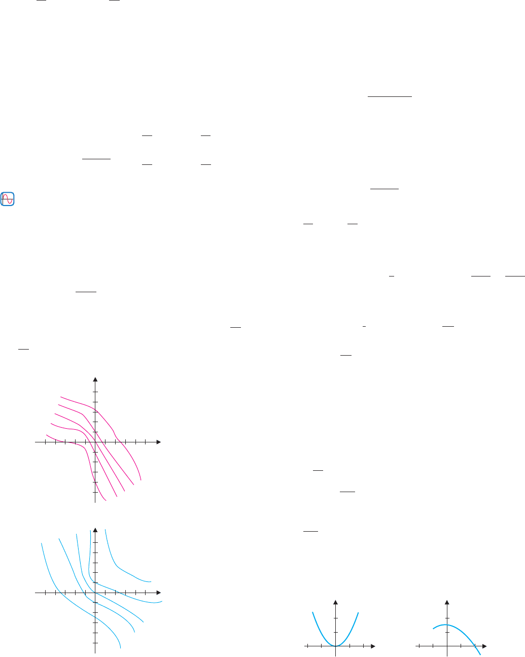
In exercises 39 and 40, use the contour plot to estimate
∂ f
∂x
and
∂ f
∂y
at (a) (0, 0), (b) (0, 1), (c) (2, 0).
39.
y
x
55
5
5
2
4
6
8
10
40.
y
x
55
5
5
2
4
6
8
10
............................................................
41. Carefullywritedownadefinitionforthethreefirst-orderpartial
derivatives of a function of three variables f (x, y, z).
42. Determine how many second-order partial derivatives there
are of f (x, y, z). Assuming a result analogous to Theorem
3.1, how many of these second-order partial derivatives are
actually different?
43. For the function
f (x, y) =
⎧
⎨
⎩
xy(x
2
− y
2
)
x
2
+ y
2
, if (x, y) = (0, 0)
0, if (x, y) = (0, 0)
use the limit definitions of partial derivatives to show that
f
xy
(0, 0) =−1but f
yx
(0, 0) = 1. Determine which assump-
tion in Theorem 3.1 is not true.
44. For f (x, y) =
⎧
⎨
⎩
xy
2
x
2
+ y
4
, if(x, y) = (0, 0)
0, if(x, y) = (0, 0)
, show that
∂ f
∂x
(0, 0) =
∂ f
∂y
(0, 0) = 0. [Note that we have previously
shown that this function is not continuous at (0, 0).]
45. Sometimes the order of differentiation makes a practical dif-
ference. For f (x, y) =
1
x
sin(xy
2
), show that
∂
2
f
∂x∂ y
=
∂
2
f
∂y∂ x
but that the ease of calculations is not the same.
46. For a rectangle of length L and perimeter P, show that the area
is given by A =
1
2
LP − L
2
. Compute
∂ A
∂ L
. A simpler formula
for area is A = LW, where W is the width of the rectangle.
Compute
∂ A
∂ L
and show that your answer is not equivalent
to the previous derivative. Explain the difference by noting
that in one case the width is held constant while L changes,
whereas in the other case the perimeter is held constant while
L changes.
47. Suppose that f (x, y) is a function with continuous second-
order partial derivatives. Consider the curve obtained by
intersecting the surface z = f (x, y) with the plane y = y
0
.
Explain how the slope of this curve at the point x = x
0
relates
to
∂ f
∂x
(x
0
, y
0
). Relate the concavity of this curve at the point
x = x
0
to
∂
2
f
∂x
2
(x
0
, y
0
).
48. As in exercise 47, develop a graphical interpretation of
∂
2
f
∂y
2
(x
0
, y
0
).
49. Given the cross sections of z = f (x, y), estimate (a) f
x
(1, 1),
(b) f
x
(0, 1), (c) f
y
(1, 0) and (d) f
y
(1, 1).
z
x
at y 1 at x 1
z
y