Thomas M. Cover, Joy A. Thomas. Elements of information theory

Подождите немного. Документ загружается.

9.1 GAUSSIAN CHANNEL: DEFINITIONS 265

Remark We ﬁrst present a plausibility argument as to why we may be

able to construct (2

,n) codes with a low probability of error. Consider

any codeword of length n. The received vector is normally distributed with

mean equal to the true codeword and variance equal to the noise variance.

With high probability, the received vector is contained in a sphere of radius

√

n(N +) around the true codeword. If we assign everything within this

sphere to the given codeword, when this codeword is sent there will be

an error only if the received vector falls outside the sphere, which has

low probability.

Similarly, we can choose other codewords and their corresponding

decoding spheres. How many such codewords can we choose? The vol-

ume of an n-dimensional sphere is of the form C

,wherer is the

radius of the sphere. In this case, each decoding sphere has radius

√

nN.

These spheres are scattered throughout the space of received vectors. The

received vectors have energy no greater than n(P + N), so they lie in a

sphere of radius

√

n(P + N). The maximum number of nonintersecting

decoding spheres in this volume is no more than

(n(P + N))

(nN)

= 2

log



1 +



(9.22)

and the rate of the code is

log(1 +

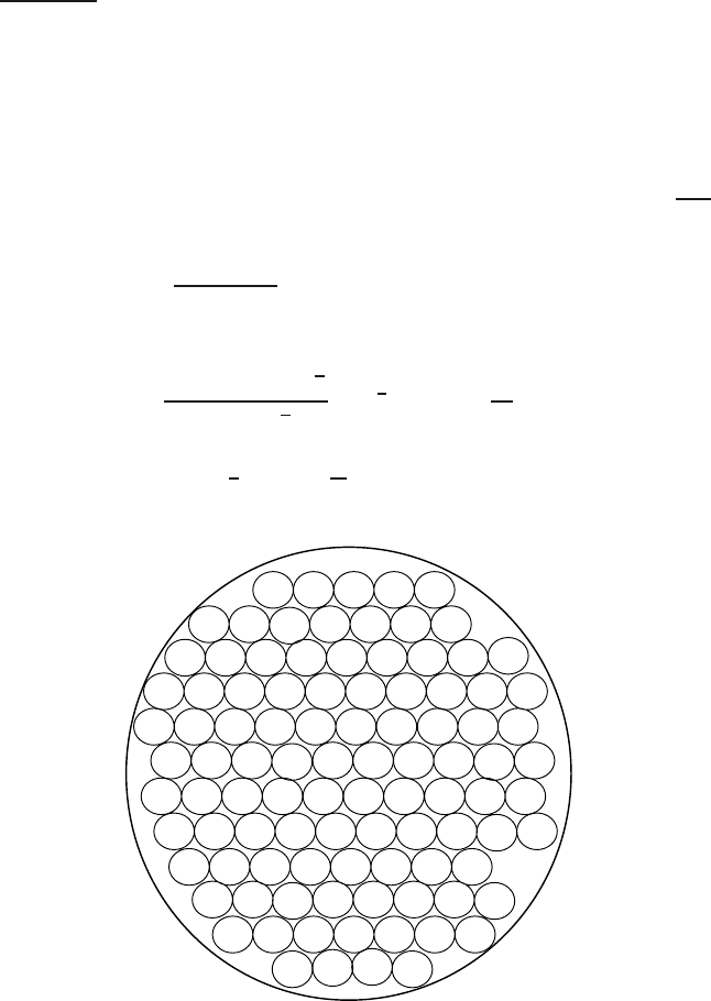
). This idea is illustrated in Figure 9.2.

FIGURE 9.2. Sphere packing for the Gaussian channel.

266 GAUSSIAN CHANNEL

This sphere-packing argument indicates that we cannot hope to send

at rates greater than C with low probability of error. However, we can

actually do almost as well as this, as is proved next.

Proof: (Achievability). We will use the same ideas as in the proof of

the channel coding theorem in the case of discrete channels: namely,

random codes and joint typicality decoding. However, we must make

some modiﬁcations to take into account the power constraint and the fact

that the variables are continuous and not discrete.

1. Generation of the codebook. We wish to generate a codebook in

which all the codewords satisfy the power constraint. To ensure

this, we generate the codewords with each element i.i.d. accord-

ing to a normal distribution with variance P − . Since for large



→ P − , the probability that a codeword does not sat-

isfy the power constraint will be small. Let X

(w), i = 1, 2,...,n,

w = 1, 2,...,2

be i.i.d. ∼ N(0,P − ), forming codewords

(1), X

(2),...,X

) ∈ R

2. Encoding. After the generation of the codebook, the codebook is

revealed to both the sender and the receiver. To send the message

index w, the transmitter sends the wth codeword X

(w) in the code-

book.

3. Decoding. The receiver looks down the list of codewords {X

(w)}

and searches for one that is jointly typical with the received vector.

If there is one and only one such codeword X

(w), the receiver

declares

W = w to be the transmitted codeword. Otherwise, the

receiver declares an error. The receiver also declares an error if the

chosen codeword does not satisfy the power constraint.

4. Probability of error . Without loss of generality, assume that code-

word 1 was sent. Thus, Y

= X

(1) + Z

. Deﬁne the following

events:









j=1

(1)>P







(9.23)

and



(i), Y

)isinA

(n)





. (9.24)

Then an error occurs if E

occurs (the power constraint is violated)

or E

occurs (the transmitted codeword and the received sequence

are not jointly typical) or E

∪ E

∪···∪E

occurs (some wrong

9.1 GAUSSIAN CHANNEL: DEFINITIONS 267

codeword is jointly typical with the received sequence). Let E denote

the event

W = W and let P denote the conditional probability given

that W = 1. Hence,

Pr(

E|W = 1) = P(E) = P



∪ E

∪···∪E



(9.25)

≤ P(E

) + P(E

) +



i=2

P(E

), (9.26)

by the union of events bound for probabilities. By the law of large

numbers, P(E

) → 0asn →∞. Now, by the joint AEP (which

can be proved using the same argument as that used in the discrete

case), P(E

) → 0, and hence

P(E

) ≤  for n sufﬁciently large. (9.27)

Since by the code generation process, X

(1) and X

(i) are indepen-

dent, so are Y

and X

(i). Hence, the probability that X

(i) and Y

will be jointly typical is ≤ 2

−n(I (X;Y)−3)

by the joint AEP.

Now let W be uniformly distributed over {1, 2,...,2

}, and con-

sequently,

Pr(

E) =



= P

(n)

. (9.28)

Then

(n)

= Pr(E) = Pr(E|W = 1) (9.29)

≤ P(E

) + P(E

) +



i=2

P(E

) (9.30)

≤  +  +



i=2

−n(I (X;Y)−3)

(9.31)

= 2 +



− 1



−n(I (X;Y)−3)

(9.32)

≤ 2 + 2

3n

−n(I (X;Y)−R)

(9.33)

≤ 3 (9.34)

268 GAUSSIAN CHANNEL

for n sufﬁciently large and R<I(X;Y)− 3. This proves the exis-

tence of a good (2

,n) code.

Now choosing a good codebook and deleting the worst half of the

codewords, we obtain a code with low maximal probability of error. In

particular, the power constraint is satisﬁed by each of the remaining code-

words (since the codewords that do not satisfy the power constraint have

probability of error 1 and must belong to the worst half of the codewords).

Hence we have constructed a code that achieves a rate arbitrarily close to

capacity. The forward part of the theorem is proved. In the next section

we show that the achievable rate cannot exceed the capacity.



9.2 CONVERSE TO THE CODING THEOREM FOR GAUSSIAN

CHANNELS

In this section we complete the proof that the capacity of a Gaussian

channel is C =

log(1 +

) by proving that rates R>Care not achiev-

able. The proof parallels the proof for the discrete channel. The main new

ingredient is the power constraint.

Proof: (Converse to Theorem 9.1.1). We must show that if P

(n)

→ 0for

a sequence of (2

,n)codes for a Gaussian channel with power constraint

P ,then

R ≤ C =

log



1 +



. (9.35)

Consider any (2

,n) code that satisﬁes the power constraint, that is,



i=1

(w) ≤ P, (9.36)

for w = 1, 2,...,2

. Proceeding as in the converse for the discrete case,

let W be distributed uniformly over {1, 2,...,2

}. The uniform distri-

bution over the index set W ∈{1, 2,...,2

} induces a distribution on

the input codewords, which in turn induces a distribution over the input

alphabet. This speciﬁes a joint distribution on W → X

(W ) → Y

→

W .

To relate probability of error and mutual information, we can apply Fano’s

inequality to obtain

H(W|

W) ≤ 1 + nRP

(n)

= n

, (9.37)

9.2 CONVERSE TO THE CODING THEOREM FOR GAUSSIAN CHANNELS 269

where 

→ 0asP

(n)

→ 0. Hence,

nR = H(W) = I(W;

W)+ H(W|

W) (9.38)

≤ I(W;

W)+ n

(9.39)

≤ I(X

) + n

(9.40)

= h(Y

) − h(Y

) + n

(9.41)

= h(Y

) − h(Z

) + n

(9.42)

≤



i=1

h(Y

) − h(Z

) + n

(9.43)



i=1

h(Y

) −



i=1

h(Z

) + n

(9.44)



i=1

I(X

) + n

. (9.45)

Here X

= x

(W ),whereW is drawn according to the uniform distribution

on {1, 2,...,2

}.NowletP

be the average power of the ith column of

the codebook, that is,



(w). (9.46)

Then, since Y

= X

+ Z

and since X

and Z

are independent, the aver-

age power EY

of Y

is P

+ N . Hence, since entropy is maximized by

the normal distribution,

h(Y

) ≤

log 2πe(P

+ N). (9.47)

Continuing with the inequalities of the converse, we obtain

nR ≤



(

h(Y

) − h(Z

)

+ n

(9.48)

≤





log(2πe(P

+ N)) −

log 2πeN



+ n

(9.49)



log



1 +



+ n

. (9.50)

270 GAUSSIAN CHANNEL

Since each of the codewords satisﬁes the power constraint, so does their

average, and hence



≤ P. (9.51)

Since f(x) =

log(1 +x) is a concave function of x, we can apply

Jensen’s inequality to obtain



i=1

log



1 +



≤

log



1 +



i=1



(9.52)

≤

log



1 +



. (9.53)

Thus R ≤

log(1 +

) + 

, 

→ 0, and we have the required converse.

Note that the power constraint enters the standard proof in (9.46).

9.3 BANDLIMITED CHANNELS

A common model for communication over a radio network or a telephone

line is a bandlimited channel with white noise. This is a continuous-

time channel. The output of such a channel can be described as the

convolution

Y(t) =

(

X(t) +Z(t)

)

∗ h(t), (9.54)

where X(t) is the signal waveform, Z(t) is the waveform of the white

Gaussian noise, and h(t ) is the impulse response of an ideal bandpass

ﬁlter, which cuts out all frequencies greater than W .Inthissectionwe

give simpliﬁed arguments to calculate the capacity of such a channel.

We begin with a representation theorem due to Nyquist [396] and Shan-

non [480], which shows that sampling a bandlimited signal at a sampling

rate

is sufﬁcient to reconstruct the signal from the samples. Intuitively,

this is due to the fact that if a signal is bandlimited to W , it cannot change

by a substantial amount in a time less than half a cycle of the maximum

frequency in the signal, that is, the signal cannot change very much in

time intervals less than

seconds.

9.3 BANDLIMITED CHANNELS 271

Theorem 9.3.1 Suppose that a function f(t) is bandlimited to W ,

namely, the spectrum of the function is 0 for all frequencies greater than

W . Then the function is completely determined by samples of the function

spaced

seconds apart.

Proof: Let F(ω) be the Fourier transform of f(t).Then

f(t)=

2π



∞

−∞

F(ω)e

iωt

dω (9.55)

2π



2πW

−2πW

F(ω)e

iωt

dω, (9.56)

since F(ω) is zero outside the band −2πW ≤ ω ≤ 2πW. If we consider

samples spaced

seconds apart, the value of the signal at the sample

points can be written





2π



2πW

−2πW

F(ω)e

iω

dω. (9.57)

The right-hand side of this equation is also the deﬁnition of the coefﬁcients

of the Fourier series expansion of the periodic extension of the function

F(ω), taking the interval −2πW to 2πW as the fundamental period. Thus,

thesamplevaluesf(

) determine the Fourier coefﬁcients and, by exten-

sion, they determine the value of F(ω) in the interval (−2πW,2πW).

Since a function is uniquely speciﬁed by its Fourier transform, and since

F(ω) is zero outside the band W , we can determine the function uniquely

from the samples.

Consider the function

sinc(t) =

sin(2πWt)

2πWt

. (9.58)

This function is 1 at t = 0andis0fort = n/2W , n = 0. The spectrum

of this function is constant in the band (−W,W) and is zero outside this

band. Now deﬁne

g(t) =

∞



n=−∞





sinc



t −



. (9.59)

From the properties of the sinc function, it follows that g(t) is bandlim-

ited to W and is equal to f(n/2W) at t = n/2W . Since there is only

272 GAUSSIAN CHANNEL

one function satisfying these constraints, we must have g(t) = f(t).This

provides an explicit representation of f(t) in terms of its samples.



A general function has an inﬁnite number of degrees of freedom—the

value of the function at every point can be chosen independently. The

Nyquist–Shannon sampling theorem shows that a bandlimited function

has only 2W degrees of freedom per second. The values of the function

at the sample points can be chosen independently, and this speciﬁes the

entire function.

If a function is bandlimited, it cannot be limited in time. But we can

consider functions that have most of their energy in bandwidth W and

have most of their energy in a ﬁnite time interval, say (0,T). We can

describe these functions using a basis of prolate spheroidal functions.We

do not go into the details of this theory here; it sufﬁces to say that there

are about 2TW orthonormal basis functions for the set of almost time-

limited, almost bandlimited functions, and we can describe any function

within the set by its coordinates in this basis. The details can be found

in a series of papers by Landau, Pollak, and Slepian [340, 341, 500].

Moreover, the projection of white noise on these basis vectors forms

an i.i.d. Gaussian process. The above arguments enable us to view the

bandlimited, time-limited functions as vectors in a vector space of 2TW

dimensions.

Now we return to the problem of communication over a bandlimited

channel. Assuming that the channel has bandwidth W , we can represent

both the input and the output by samples taken 1/2W seconds apart. Each

of the input samples is corrupted by noise to produce the corresponding

output sample. Since the noise is white and Gaussian, it can be shown

that each noise sample is an independent, identically distributed Gaussian

random variable.

If the noise has power spectral density N

/2 watts/hertz and bandwidth

W hertz, the noise has power

2W = N

W and each of the 2WT noise

samples in time T has variance N

WT/2WT = N

/2. Looking at the

input as a vector in the 2TW-dimensional space, we see that the received

signal is spherically normally distributed about this point with covariance

I .

Now we can use the theory derived earlier for discrete-time Gaussian

channels, where it was shown that the capacity of such a channel is

C =

log



1 +



bits per transmission. (9.60)

Let the channel be used over the time interval [0,T]. In this case, the

energy per sample is PT/2WT = P/2W , the noise variance per sample

9.3 BANDLIMITED CHANNELS 273

2WT

= N

/2, and hence the capacity per sample is

C =

log



1 +



log



1 +



bits per sample.

(9.61)

Since there are 2W samples each second, the capacity of the channel can

be rewritten as

C = W log



1 +



bits per second. (9.62)

This equation is one of the most famous formulas of information theory. It

gives the capacity of a bandlimited Gaussian channel with noise spectral

density N

/2 watts/Hz and power P watts.

A more precise version of the capacity argument [576] involves con-

sideration of signals with a small fraction of their energy outside the

bandwidth W of the channel and a small fraction of their energy outside

the time interval (0,T). The capacity above is then obtained as a limit as

the fraction of energy outside the band goes to zero.

If we let W →∞in (9.62), we obtain

C =

log

e bits per second (9.63)

as the capacity of a channel with an inﬁnite bandwidth, power P ,and

noise spectral density N

/2. Thus, for inﬁnite bandwidth channels, the

capacity grows linearly with the power.

Example 9.3.1 (Telephone line) To allow multiplexing of many chan-

nels, telephone signals are bandlimited to 3300 Hz. Using a bandwidth of

3300 Hz and a SNR (signal-to-noise ratio) of 33 dB (i.e., P/N

W =

2000) in (9.62), we ﬁnd the capacity of the telephone channel to be

about 36,000 bits per second. Practical modems achieve transmission rates

up to 33,600 bits per second in both directions over a telephone channel.

In real telephone channels, there are other factors, such as crosstalk, inter-

ference, echoes, and nonﬂat channels which must be compensated for to

achieve this capacity.

The V.90 modems that achieve 56 kb/s over the telephone channel

achieve this rate in only one direction, taking advantage of a purely digital

channel from the server to ﬁnal telephone switch in the network. In this

case, the only impairments are due to the digital-to-analog conversion at

this switch and the noise in the copper link from the switch to the home;

274 GAUSSIAN CHANNEL

these impairments reduce the maximum bit rate from the 64 kb/s for the

digital signal in the network to the 56 kb/s in the best of telephone lines.

The actual bandwidth available on the copper wire that links a home to

a telephone switch is on the order of a few megahertz; it depends on the

length of the wire. The frequency response is far from ﬂat over this band.

If the entire bandwidth is used, it is possible to send a few megabits per

second through this channel; schemes such at DSL (Digital Subscriber

Line) achieve this using special equipment at both ends of the telephone

line (unlike modems, which do not require modiﬁcation at the telephone

switch).

9.4 PARALLEL GAUSSIAN CHANNELS

In this section we consider k independent Gaussian channels in parallel

with a common power constraint. The objective is to distribute the total

power among the channels so as to maximize the capacity. This channel

models a nonwhite additive Gaussian noise channel where each parallel

component represents a different frequency.

Assume that we have a set of Gaussian channels in parallel as illustrated

in Figure 9.3. The output of each channel is the sum of the input and

Gaussian noise. For channel j ,

= X

+ Z

,j= 1, 2,...,k, (9.64)

with

∼ N(0,N

), (9.65)

and the noise is assumed to be independent from channel to channel. We

assume that there is a common power constraint on the total power used,

that is,



j=1

≤ P. (9.66)

We wish to distribute the power among the various channels so as to

maximize the total capacity.

The information capacity of the channel C is

C = max

f(x

,...,x



≤P

I(X

,...,X

; Y

,...,Y

). (9.67)