Townsend C.R., Begon M., Harper J.L. Essentials of Ecology

Подождите немного. Документ загружается.

had previously eaten between them – as did the rodents when the ants were

removed; only when both were removed did the amount of resource increase.

In other words, under normal circumstances both guilds eat less and achieve

lower levels of abundance than they would do if the other guild were absent. This

clearly indicates that rodents and ants, although they coexist in the same habitat,

compete interspeciﬁcally with one another.

6.2.7 The Competitive Exclusion Principle

The patterns that are apparent in these examples have also been uncovered in

many others, and have been elevated to the status of a principle: the Competitive

Exclusion Principle or Gause’s Principle (named after an eminent Russian ecologist).

It can be stated as follows:

If two competing species coexist in a stable environment, then they

do so as a result of niche differentiation, i.e. differentiation of their

realized niches.

If, however, there is no such differentiation, or if it is precluded by the

habitat, then one competing species will eliminate or exclude the other.

Although the principle has emerged here from a contemplation of patterns

evident in real sets of data, its establishment was – and many modern discussions

of interspeciﬁc competition still are – bound up with a simple mathematical model

of interspeciﬁc competition, usually known by the names of its two (independent)

originators: Lotka and Volterra (Box 6.1).

There is no question that there is some truth in the principle that competitor

species can coexist as a result of niche differentiation, and that one competitor

species may exclude another by denying it a realized niche. But it is crucial also

to be aware of what the Competitive Exclusion Principle does not say.

It does not say that whenever we see coexisting species with different niches

it is reasonable to jump to the conclusion that this is the principle in operation.

Each species, on close inspection, has its own unique niche. Niche differentiation

Chapter 6 Interspeciﬁc competition

189

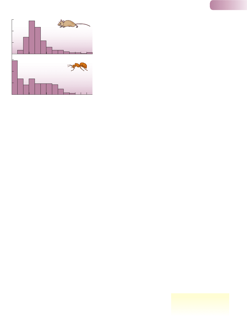
Figure 6.5

The diets of ants and rodents overlap:

sizes of seeds harvested by coexisting

ants and rodents near Portal, Arizona.

AFTER BROWN & DAVIDSON, 1977

0.3

0.2

0.1

0.0

0.3

0.2

0.1

0.0

<0.64

0.64–0.70

0.70–0.83

0.83–0.99

0.99–1.17

1.17–1.40

1.40–1.85

1.85–1.98

1.98–2.36

2.36–2.79

2.79–3.33

3.33–3.96

3.96–4.70

>4.70

Seed size (mm)

Frequency in diet

Rodents

Ants

The Competitive Exclusion

Principle – what it does and

does not say

9781405156585_4_006.qxd 11/5/07 14:51 Page 189

Part III Individuals, Populations, Communities and Ecosystems

190

(a) (b)

/α

6.1 QUANTITATIVE ASPECTS

6.1 Quantitative aspects

The most widely used model of interspeciﬁc competi-

tion is the Lotka–Volterra model (Volterra, 1926; Lotka,

1932). It is an extension of the logistic equation described

in Box 5.4. Its virtues are (like the logistic) its simplicity,

and its capacity to shed light on the factors that deter-

mine the outcome of a competitive interaction.

Within the logistic equation,

= rN

the particular term that models intraspeciﬁc competi-

tion is (K − N)/K. Within this term, the greater the value

of N (the bigger the population), the greater is the

strength of intraspeciﬁc competition. The basis of the

Lotka–Volterra model is the replacement of this term

by one that models both intra- and interspeciﬁc com-

petition. In the model, we call the population size of

the ﬁrst species N

, and that of a second species N

Their carrying capacities and intrinsic rates of increase

are K

, K

, r

and r

By analogy with the logistic, we expect the total

competitive effect on, say, species 1 (intra- and inter-

speciﬁc) to be greater the larger the values of N

and

; but we cannot just add them together, since the

competitive effects of the two species on species 1

are unlikely to be the same. Suppose, though, that

10 individuals of species 2 have, between them, only

the same competitive effect on species 1 as does a

single individual of species 1. The total competitive

effect on species 1 will then be equivalent to the effect

of (N

+ N

1/10) species 1 individuals. The constant

(1/10 in the present case) is called a competition

coefﬁcient and is denoted by α

(alpha one two).

Multiplying N

by α

converts it to a number of N

equivalents, and adding N

and α

together gives

us the total competitive effect on species 1. (Note

that α

< 1 means that individuals of species 2 have

less inhibitory effect on individuals of species 1 than

individuals of species 1 have on others of their own

species, and so on.)

(K − N)

The equation for species 1 can now be written:

= r

and for species 2 (with its own competition coefﬁcient,

converting species 1 individuals into species 2

equivalents):

= r

These two equations constitute the Lotka–Volterra

model.

The best way to appreciate its properties is to ask

the question, ‘Under what circumstances does each

species increase or decrease in abundance?’ In order

to answer, it is necessary to construct diagrams in

which all possible combinations of N

and N

can be

displayed. This has been done in Figure 6.6. Certain

combinations (certain regions in Figure 6.6) give rise

to increases in species 1 and/or species 2, whereas

other combinations give rise to decreases. It follows

inevitably that there must also therefore be a so-called

− [N

+ α

])

− [N

+ α

])

The Lotka–Volterra model of interspeciﬁc competition

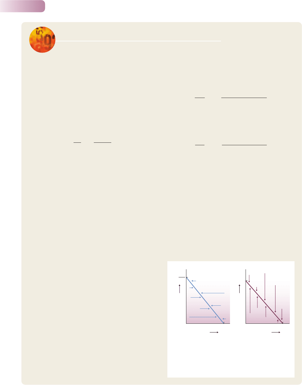
Figure 6.6

The zero isoclines generated by the Lotka–Volterra

competition equations. (a) The N

zero isocline: species 1

increases below and to the left of it, and decreases above

and to the right of it. (b) The equivalent N

isocline.

9781405156585_4_006.qxd 11/5/07 14:51 Page 190

Chapter 6 Interspeciﬁc competition

191

zero isocline for each species: that is, a line with com-

binations leading to increase on one side of it and

combinations leading to decrease on the other, but

along which there is neither increase nor decrease.

We can map out the regions of increase and

decrease in Figure 6.6 for species 1 if we can draw its

zero isocline, and we can do this by using the fact that

on the zero isocline, dN

/dt = 0 (the rate of change of

species 1 abundance is zero, by deﬁnition). Rearrang-

ing the equation, this gives us, as the zero isocline for

species 1:

= K

− α

Below and to the left of this, species 1 increases

in abundance (arrows in the ﬁgure, representing this

increase, point from left to right, since N

is on the

horizontal axis). It increases because numbers of

both species are relatively low, and species 1 is thus

subjected to only weak competition. Above and to the

right of the line, however, numbers are high, competi-

tion is strong and species 1 decreases in abundance

(arrows from right to left). Based on an equivalent

derivation, Figure 6.6b also shows the species 2 zero

isocline, with arrows, like the N

axis, running vertically.

In order to determine the outcome of competition

in this model, it is necessary to determine, at each

point on a ﬁgure, the behavior of the joint species

1–species 2 population, as indicated by the pair of

arrows. There are, in fact, four different ways in which

the two zero isoclines can be arranged relative to one

another, and these can be distinguished by the inter-

cepts of the zero isoclines (Figure 6.7). The outcome

of competition will be different in each case.

Looking at the intercepts in Figure 6.7a, for

instance,

> K

and K

Rearranging these slightly gives us:

> K

and K

> K

The ﬁrst inequality (K

> K

) indicates that the

inhibitory intraspeciﬁc effects that species 1 can exert

on itself (denoted by K

) are greater than the inter-

speciﬁc effects that species 2 can exert on species 1

). This means that species 2 is a weak inter-

speciﬁc competitor. The second inequality, however,

indicates that species 1 can exert more of an effect

/α

(a) (b)

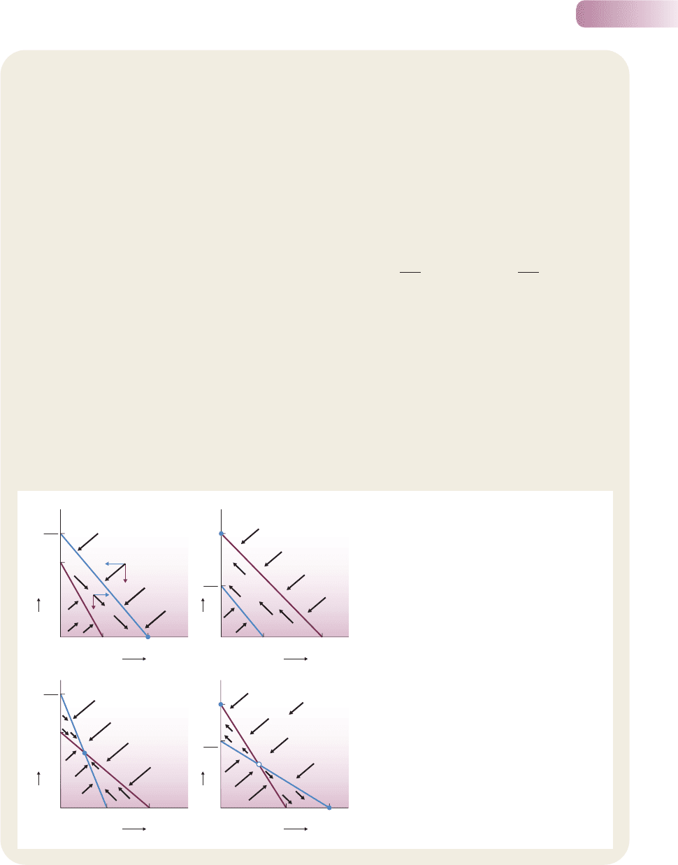
Figure 6.7

The outcomes of competition generated by the

Lotka–Volterra competition equations for the four

possible arrangements of the N

and N

zero

isoclines. Black arrows refer to joint populations,

and are derived as indicated in (a). The solid circles

show stable equilibrium points. The open circle in

(d) is an unstable equilibrium point. For further

discussion, see box text.

9781405156585_4_006.qxd 11/5/07 14:51 Page 191

does not prove that there are coexisting competitors. The species may not be

competing at all and may never have done so in their evolutionary history. We

require proof of interspeciﬁc competition. In the examples above, this was provided

by experimental manipulation – remove one species (or one group of species)

and the other species increases its abundance or its survival. But most of even the

more plausible cases for competitors coexisting as a result of niche differentia-

tion have not been subjected to experimental proof. So just how important is

the Competitive Exclusion Principle in practice? We return to this question in

Section 6.5.

Part of the problem is that although species may not be competing now, their

ancestors may have competed in the past, so that the mark of interspeciﬁc com-

petition is left imprinted on the niches, the behavior or the morphology of their

present-day descendants. This particular question is taken up in Section 6.3.

Finally, the Competitive Exclusion Principle, as stated above, includes the

word ‘stable’. That is, in the habitats envisaged in the principle, conditions and

the supply of resources remain more or less constant – if species compete, then

that competition runs its course, either until one of the species is eliminated

or until the species settle into a pattern of coexistence within their realized

niches. Sometimes this is a realistic view of a habitat, especially in laboratory

Part III Individuals, Populations, Communities and Ecosystems

192

on species 2 than species 2 can on itself. Species 1

is thus a strong interspeciﬁc competitor; and as the

arrows in Figure 6.7a show, species 1 drives the weak

species 2 to extinction and attains its own carrying

capacity. The situation is reversed in Figure 6.7b.

Hence Figure 6.7a and b describe cases in which

the environment is such that one species invariably

outcompetes the other, because the ﬁrst is a strong

interspeciﬁc competitor and the other weak.

In Figure 6.7c, by contrast:

> K

and K

> K

In this case, both species have less competitive

effect on the other species than those other species

have on themselves; in this sense, both are weak

competitors. This would happen, for example, if there

were niche differentiation between the species –

each competed mostly ‘within’ its own niche. The

outcome, as Figure 6.7c shows, is that all arrows point

towards a stable, equilibrium combination of the

two species, which all joint populations therefore tend

to approach: that is, the outcome of this type of com-

petition is the stable coexistence of the competitors.

Indeed, it is only this type of competition (both species

having more effect on themselves than on the other

species) that does lead to the stable coexistence of

competitors.

Finally, in Figure 6.7d:

> K

and K

> K

Thus individuals of both species have a greater com-

petitive effect on individuals of the other species than

those other species do on themselves. This will occur,

for instance, when each species is more aggressive

toward individuals of the other species than toward

individuals of its own species. The directions of the

arrows are rather more complicated in this case, but

eventually they always lead to one or other of two

alternative stable points. At the ﬁrst, species 1 reaches

its carrying capacity with species 2 extinct; at the

second, species 2 reaches its carrying capacity with

species 1 extinct. In other words, both species are

capable of driving the other species to extinction,

but which actually does so cannot be predicted with

certainty. It depends on which species has the upper

hand in terms of densities, either because they start

with a higher density or because density ﬂuctua-

tions in some other way give them that advantage.

Whichever species has this upper hand, capitalizes

on that and drives the other species to extinction.

9781405156585_4_006.qxd 11/5/07 14:51 Page 192

or other controlled environments where the experimenter holds conditions and

the supply of resources constant. However, most environments are not stable

for long periods of time. How does the outcome of competition change when

environmental heterogeneity in space and time are taken into consideration? This

is the subject of the next section.

6.2.8 Environmental heterogeneity

As explained in previous chapters, spatial and temporal variations in environ-

ments are the norm rather than the exception. Environments are usually a

patchwork of favorable and unfavorable habitats; patches are often only available

temporarily; and patches often appear at unpredictable times and in unpredict-

able places. Under such variable conditions, competition may only rarely ‘run

its course’, and the outcome cannot be predicted simply by application of the

Competitive Exclusion Principle. A species that is a ‘weak’ competitor in a con-

stant environment might, for example, be good at colonizing open gaps created

in a habitat by ﬁre, or a storm, or the hoofprint of a cow in the mud – or may be

good at growing rapidly in such gaps immediately after they are colonized. It

may then coexist with a strong competitor, as long as new gaps occur frequently

enough. Thus, a realistic view of interspeciﬁc competition must acknowledge that

it often proceeds not in isolation, but under the inﬂuence of, and within the

constraints of, a patchy, impermanent or unpredictable world.

The following examples illustrate just two of the many ways in which environ-

mental heterogeneity ensures that the Competitive Exclusion Principle is very far

from being the whole story when it comes to determining the outcome of an

interaction between competing species.

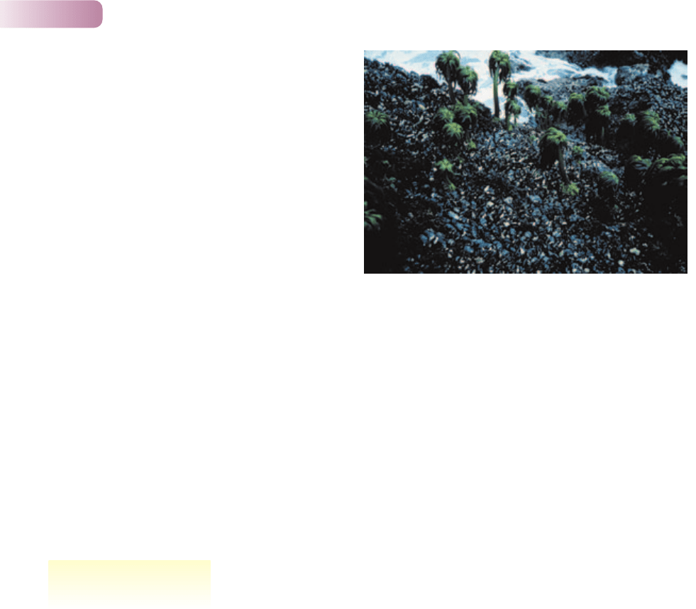
The ﬁrst concerns the coexistence of a superior competitor and a superior

colonizer: the sea palm Postelsia palmaeformis (a brown alga) and the mussel

Mytilus californianus on the coast of Washington, USA (Paine, 1979) (Figure 6.8).

Chapter 6 Interspeciﬁc competition

193

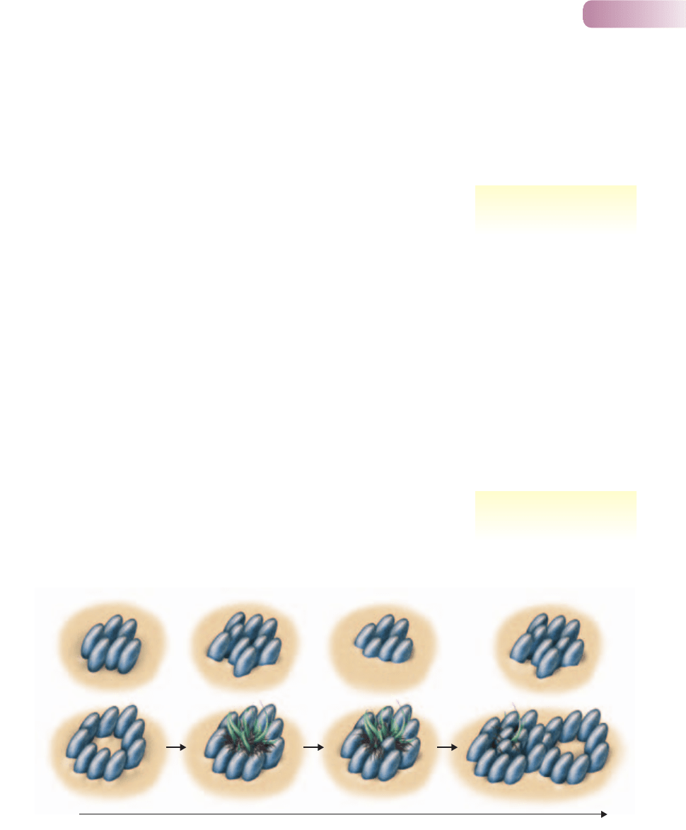
Time

Low

disturbance

shore

Regularly

disturbed

shore

Figure 6.8

On shores in which gaps are not created, mussels are able to exclude the brown alga Postelsia; but where gaps are created regularly enough the

two species coexist, even though Postelsia is eventually excluded by the mussels from each gap.

competition may only rarely

‘run its course’

mussels, sea palms and the

frequency of gap formation

9781405156585_4_006.qxd 11/5/07 14:51 Page 193

Postelsia is an annual plant that must re-establish itself each year in order to persist

at a site. It does so by attaching to the bare rock, usually in gaps in the mussel bed

created by wave action. However, the mussels themselves slowly encroach on

these gaps, gradually ﬁlling them and precluding colonization by Postelsia. In

other words, in a stable environment, the mussels would outcompete and exclude

Postelsia. But their environment is not stable – gaps are frequently being created.

It turns out that these species coexist only at sites in which there is a relatively

high average rate of gap formation (at least 7% of surface area per year), and in

which this rate is approximately the same each year. Where the average rate is

lower, or where it varies considerably from year to year, there is (either regularly

or occasionally) a lack of bare rock for colonization by Postelsia. At the sites of

coexistence, on the other hand, although Postelsia is eventually excluded from

each gap, these are created with sufﬁcient frequency and regularity for there to

be coexistence in the site as a whole. In short, there is coexistence of competitors

– but not as a result of niche differentiation.

A perhaps more widespread path to the coexistence of a superior and an

inferior competitor is based on the idea that the two species may have independ-

ent, aggregated (i.e. clumped) distributions over the available habitat. This would

mean that the powers of the superior competitor were mostly directed against

members of its own species (in the high-density clumps), but that this aggregated

superior competitor would be absent from many areas – within which the inferior

competitor could escape competition. An inferior competitor may then be able

to coexist with a superior competitor that would rapidly exclude it from a con-

tinuous, homogeneous environment.

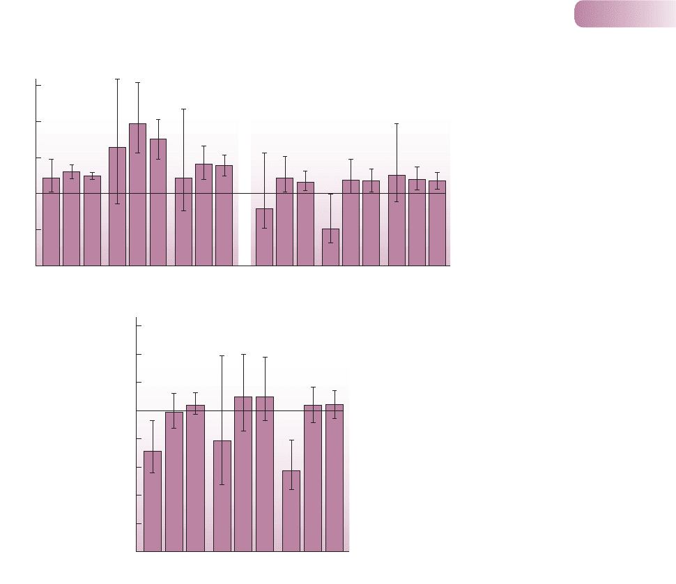
That such aggregated distributions are indeed a reality is illustrated by a ﬁeld

study of two species of sand-dune plant, Aira praecox and Erodium cicutarium,

in northwest England. Both species were aggregated, and the smaller plant, Aira,

tended to be aggregated even at the smallest spatial scales (Figure 6.9a). The two

species, though, were negatively associated with one another at these smallest

scales (Figure 6.9b). Thus, Aira tended to occur in small single-species clumps

and was therefore much less liable to competition from Erodium than would have

been the case if they had been distributed at random.

The consequences of such aggregated distributions are illustrated by a

study of experimental communities of four annual terrestrial plants – Capsella

Part III Individuals, Populations, Communities and Ecosystems

194

Seashore with Postelsia

and Mytilus californianus.

coexistence as a result of

aggregated distributions

9781405156585_4_006.qxd 11/5/07 14:51 Page 194

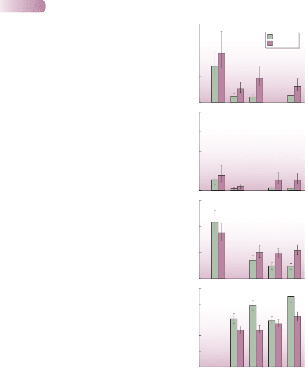
bursa-pastoris, Cardamine hirsuta, Poa annua and Stellaria media (Figure 6.10).

Stellaria is known to be the superior competitor among these species. Replicate

three- and four-species mixtures were sown at high density, and the seeds were

either placed completely at random, or seeds of each species were aggregated

in subplots within the experimental areas. Intraspeciﬁc aggregation harmed the

performance of the superior Stellaria in the mixtures, whereas in all but one

case aggregation improved the performance of the three inferior competitors.

Again, coexistence of competitors was favored not by niche differentiation but

simply by a type of heterogeneity that is typical of the natural world: aggregation

ensured that most individuals competed with members of their own and not of

another species.

These studies, and others like them, go a long way toward explaining the

co-occurrence of species that in constant, homogeneous environments would

probably exclude one another. The environment is rarely unvarying enough for

competitive exclusion to run its course or for the outcome to be the same across

the landscape.

Chapter 6 Interspeciﬁc competition

195

(b)

Association index

10 30 50 10 30 50 10 30 50

1995 1996 1997

Radius (mm)

(a)

Aggregation index

0.0

1.0

2.0

0.5

1.5

2.5

30 50 10 30 50 10 30 50

1995 1996 1997

Aira

Radius (mm)

10 30 50 10 30 50 10 30 50

1995 1996 1997

Erodium

1.6

1.4

1.2

1.0

0.8

0.6

0.4

0.2

0.0

Figure 6.9

(a) Spatial distribution of two

sand-dune species, Aira praecox

and Erodium cicutarium at a site in

northwest England. An aggregation

index of 1 indicates a random

distribution. Indices greater than

1 indicate aggregation (clumping)

within patches with the radius as

speciﬁed; values less than 1 indicate

a regular distribution. Bars represent

95% conﬁdence intervals. (b) The

association between Aria and

Erodium in each of the 3 years.

An association index greater than 1

would indicate that the two species

tended to be found together more

than would be expected by chance

alone in patches with the radius as

speciﬁed; values less than 1 indicate

a tendency to ﬁnd one species or

the other. Bars represent 95%

conﬁdence intervals.

AFTER COOMES ET AL., 2002

9781405156585_4_006.qxd 11/5/07 14:51 Page 195

Part III Individuals, Populations, Communities and Ecosystems

196

900

600

300

(a)

Capsella bursa-pastoris

Random

Aggregated

100

(b)

Cardamine hirsuta

300

200

100

(c)

Poa annua

2000

1000

Mixtures

(d) Stellaria media

Above-ground biomass (g m

–2

)

Cbp

Figure 6.10

The effect of intraspeciﬁc aggregation on above-ground biomass

(mean ± SE) of four plant species grown for 6 weeks in three- and

four-species mixtures (four replicates of each). The normally competitively

superior Stellaria media (Sm) did consistently less well when seeds were

aggregated than when they were placed at random (d). In contrast, the

three competitively inferior species – Capsella bursa-pastoris (Cbp),

Cardamine hirsuta (Ch) and Poa annua (Pa) – almost always performed

better when seeds had been aggregated (a–c). Note the different scales

on the vertical axes, and that the compositions of the mixtures are given

only along the horizontal axis of (d).

AFTER STOLL & PRATI, 2001

9781405156585_4_006.qxd 11/5/07 14:51 Page 196

6.3 Evolutionary effects of interspeciﬁc

competition

Putting to one side the fact that environmental heterogeneity ensures that the

forces of interspeciﬁc competition are often much less profound than they would

otherwise be, it is nonetheless the case that the potential of interspeciﬁc com-

petition to adversely affect individuals is considerable. We have seen in Chapter 2

that natural selection in the past will have favored those individuals that, by their

behavior, physiology or morphology, have avoided adverse effects that act on

other individuals in the same population. The adverse effects of extreme cold, for

example, may have favored individuals with an enzyme capable of functioning

effectively at low temperatures. Similarly, in the present context, the adverse

effects of interspeciﬁc competition may have favored those individuals that

managed to avoid those competitive effects. We can, therefore, expect species to

have evolved characteristics that ensure that they compete less, or not at all, with

members of other species.

How will this look to us at the present time? Coexisting species, with an appar-

ent potential to compete, will exhibit differences in behavior, physiology or

morphology that ensure that they compete little or not at all. Connell has called

this line of reasoning ‘invoking the ghost of competition past’. Yet the pattern it

predicts is precisely the same as that supposed by the Competitive Exclusion

Principle to be a prerequisite for the coexistence of species that still compete.

Coexisting present-day competitors, and coexisting species that have evolved an

avoidance of competition, can look the same.

The question of how important either past or present competition are as

forces structuring natural communities will be addressed in the last section of this

chapter (Section 6.5). For now, we examine some examples of what interspeciﬁc

competition can do as an evolutionary force. Note, however, that by invoking

something that cannot be observed directly (evolution), it may be impossible

to prove an evolutionary effect of interspeciﬁc competition, in the strict sense

of ‘proof’ that can be applied to mathematical theorems or carefully controlled

experiments in the laboratory. Nonetheless, we consider some examples where

an evolutionary (rather than an ecological) effect of interspeciﬁc competition is

the most reasonable explanation for what is observed.

6.3.1 Character displacement and ecological release in

the Indian mongoose

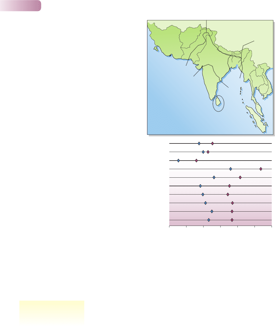
In western parts of its range, the small Indian mongoose (Herpestes javanicus)

coexists with one or two slightly larger species in the same genus (H. edwardsii

and H. smithii), but these species are absent in the eastern part of its range

(Figure 6.11a). The upper canine teeth are the mongoose’s principal prey-killing

organ, and these vary in size within and between species and between the sexes

(female mongooses are smaller than males). In the east, where H. javanicus occurs

alone (area VII in Figure 6.11a), both males and females have larger canines

than in the western areas (III, V, VI) where it coexists with the larger species

(Figure 6.11b). This is consistent with the view that where similar but larger

mongoose species are present, the prey-catching apparatus of H. javanicus has

Chapter 6 Interspeciﬁc competition

197

evolutionary avoidance of

competition

invoking the ghost of

competition past

the difﬁculty of distinguishing

ecological and evolutionary

effects

9781405156585_4_006.qxd 11/5/07 14:51 Page 197

been selected for reduced size (referred to as ‘character displacement’), reducing

the strength of competition with other species in the genus because smaller

predators tend to take smaller prey. Where H. javanicus occurs in isolation,

since no character displacement has occurred, its canine teeth are much larger.

(Another strong candidate for the evolutionary effects of interspeciﬁc competi-

tion, especially because of its association with character displacement, is provided

by Darwin’s ﬁnches of the genus Geospiza living on the Galapagos islands, dis-

cussed in Section 2.4.2.)

In fact, H. javanicus was introduced about a century ago to many islands

outside its native range (often as part of a naive attempt to control introduced

rodents). In these places, the larger competitor mongoose species were absent.

Within 100–200 generations H. javanicus had increased in size (Figure 6.11b),

so that the sizes of island individuals are now intermediate between those in the

region of origin (where they coexisted with other species and were small) and

those in the east where they occur alone. Their size on the islands is consistent

with ‘ecological release’ from competition with larger species.

Part III Individuals, Populations, Communities and Ecosystems

198

(a)

(b) Asia III

Asia VI

St Croix

Hawaii

Oahu

Mauritius

2.25 2.50 2.75 3.00 3.25 3.50 3.75

Asia V

Asia VII

Viti Levu

Okinawa

sup

L (mm)

(e, j)

III

(e, j, s)

(e, j)

(e, s)

(e, j, s)

VII

(j)

Figure 6.11

(a) Native geographic ranges of Herpestes javanicus (j),

H. edwardsii (e) and H. smithii (s). (b) Maximum diameter (mm)

of the upper canine (C

sup

L) for Herpestes javanicus in its native

range [data only for areas III, V, VI and VII from (a)] and islands on

which it has been introduced. Symbols in blue represent mean

female size and in maroon mean male size. Compared to area VII

(H. javanicus alone), animals in areas III, V and VI, where they

compete with the two larger species, are smaller. On the islands,

they have increased in size since their introduction, but are still not

as large as in area VII.

FROM SIMBERLOFF ET AL., 2000

smaller teeth in the small Indian

mongoose when larger

competitors are present

9781405156585_4_006.qxd 11/5/07 14:51 Page 198