Trauth M.H., MATLAB® Recipes for Earth Sciences, Third edition

Подождите немного. Документ загружается.

118 5 TIME-SERIES ANALYSIS

performing spectral analyses. Type help spectrum for more informa-

tion about object-oriented spectral analysis.  e non-object-oriented func-

tions to perform spectral analyses, however, are still available. One of the

oldest functions in this toolbox is

periodogram(x,window,nfft,fs)

which computes the power spectral density

Pxx of a time series x(t) using

the periodogram method.  is method was invented by Arthur Schuster

in 1898 for studying the climate, and calculates the power spectrum by

performing a Fourier transform directly on a sequence without requiring

prior calculation of the autocorrelation sequence.  e periodogram meth-

od can therefore be considered a special case of the Blackman and Tukey

(1958) method, applied with the lag parameter k set to unity (Muller and

Macdonald 2000). At the time of its introduction in 1958, the indirect com-

putation of the power spectrum via an autocorrelation sequence was faster

than calculating the Fourier transformation for the full data series

x(t) di-

rectly. A er the introduction of the Fast Fourier Transform (FFT) by Cooley

and Turkey (1965), and subsequent faster computer hardware, the higher

computing speed of the Blackman-Tukey approach compared to the peri-

odogram method became relatively unimportant.

For this next example we again use the synthetic time series

x, xn and

xt generated in Section 5.2 as the input:

clear

t = 1 : 1000; t = t';

x = 2*sin(2*pi*t/50) + sin(2*pi*t/15) + 0.5*sin(2*pi*t/5);

randn('seed',0)

n = randn(1000,1);

xn = x + n;

xt = x + 0.005*t;

We then compute the periodogram by calculating the Fourier transform of

the sequence

x.  e fastest possible Fourier transform using fft computes

the Fourier transform for

nfft frequencies, where nfft is the next power

of two closest to the number of data points

n in the original signal x. Since

the length of the data series is

n=1000, the Fourier transform is computed

for

nfft=1024 frequencies, while the signal is padded with nfft-n=24

zeros.

Xxx = fft(x,1024);

If nfft is even as in our example, then Xxx is symmetric. For example,

as the  rst

(1+nfft/2) points in Xxx are unique, the remaining points

5.4 EXAMPLES OF AUTO-SPECTRAL AND CROSS-SPECTRAL ANALYSIS 119

5 TIME-SERIES ANALYSIS

are symmetrically redundant.  e power spectral density is de ned as

Pxx2=(abs(Xxx).^2)/Fs, where Fs is the sampling frequency.  e

function

periodogram also scales the power spectral density by the length

of the data series, i. e., it divides by

Fs=1 and length(x)=1000.

Pxx2 = abs(Xxx).^2/1000;

We now drop the redundant part in the power spectrum and use only the

 rst

(1+nfft/2) points. We also multiply the power spectral density by

two to keep the same energy as in the symmetric spectrum, except for the

 rst data point.

Pxx = [Pxx2(1); 2*Pxx2(2:512)];

 e corresponding frequency axis runs from 0 to Fs/2 in Fs/(nfft-1)

steps, where

Fs/2 is the Nyquist frequency. Since Fs=1 in our example, the

frequency axis is

f = 0 : 1/(1024-1) : 1/2;

We then plot the power spectral density Pxx in the Nyquist frequency range

from

0 to Fs/2, which in our example is from 0 to 1/2.  e Nyquist fre-

quency range corresponds to the  rst 512 or

nfft/2 data points.

plot(f,Pxx), grid

 e graphical output shows that there are three signi cant peaks at the posi-

tions of the original frequencies 1/50, 1/15 and 1/5 of the three sine waves.

 e code for the power spectral density can be rewritten to make it indepen-

dent of the sampling frequency,

Fs = 1;

t = 1/Fs :1/Fs : 1000/Fs; t = t';

x = 2*sin(2*pi*t/50) + sin(2*pi*t/15) + 0.5*sin(2*pi*t/5);

nfft = 2^nextpow2(length(t));

Xxx = fft(x,nfft);

Pxx2 = abs(Xxx).^2 /Fs /length(x);

Pxx = [Pxx2(1); 2*Pxx2(2:512)];

f = 0 : Fs/(nfft-1) : Fs/2;

plot(f,Pxx), grid

axis([0 0.5 0 max(Pxx)])

where the function nextpow2 computes the next power of two closest to

the length of the time series

x(t).  is code allows the sampling frequency

120 5 TIME-SERIES ANALYSIS

to be modi ed and the di erences in the results to be explored.

We can now compare the results with those of the function

periodogram(x,window,nfft,fs).  is function allows the window-

ing of the signals with various window shapes to overcome spectral leakage.

We use, however, the default rectangular window by choosing an empty

vector

[] for window to compare the results with the above experiment.

 e power spectrum

Pxx is computed using a FFT of length nfft=1024

which is the next power of two closest to the length of the series x(t), and

which is padded with zeros to make up the number of data points to the

value of

nfft. A sampling frequency fs of one is used within the function

in order to obtain the correct frequency scaling for the f-axis.

[Pxx,f] = periodogram(x,[],1024,1);

plot(f,Pxx), grid

xlabel('Frequency')

ylabel('Power')

title('Auto-Spectrum')

 e graphical output is almost identical to our Blackman-Tukey plot and

again shows that there are three signi cant peaks at the position of the orig-

inal frequencies of the three sine waves.  e same procedure can also be

applied to the noisy data:

[Pxx,f] = periodogram(xn,[],1024,1);

plot(f,Pxx), grid

xlabel('Frequency')

ylabel('Power')

title('Auto-Spectrum')

Let us now increase the noise level by using Gaussian noise with a standard

deviation of  ve and zero mean.

randn('seed',0);

n = 5 * randn(size(x));

xn = x + n;

[Pxx,f] = periodogram(xn,[],1024,1);

plot(f,Pxx), grid

xlabel('Frequency')

ylabel('Power')

title('Auto-Spectrum')

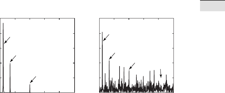
 is spectrum resembles a real data spectrum in the earth sciences.  e

spectral peaks now sit on a signi cant background noise level.  e peak of

the highest frequency even disappears into the noise, and cannot be dis-

tinguished from maxima that are attributed to noise. Both spectra can be

5.4 EXAMPLES OF AUTO-SPECTRAL AND CROSS-SPECTRAL ANALYSIS 121

5 TIME-SERIES ANALYSIS

Power

=0.02

≈0.07

=0.2

=0.02

≈0.07

=0.2 ?

Noise

oor

0.2

0.3

0.4

0.5

0.1

200

400

600

800

1000

200

400

600

800

1000

0.2

0.3

0.4

0.5

0.1

Frequency Frequency

Autospectrum Autospectrum

Fig. 5.6 Comparison of the auto-spectra for a the noise-free and b the noisy synthetic signals

with the periods τ

=50 ( f

=0.02), τ

=15 (f

≈0.07) and τ

=5 (f

=0.2). In particular, the

highest frequency peak disappears into the background noise and cannot be distinguished

from peaks attributed to the Gaussian noise.

compared on the same plot (Fig. 5.6):

[Pxx,f] = periodogram(x,[],1024,1);

[Pxxn,f] = periodogram(xn,[],1024,1);

subplot(1,2,1)

plot(f,Pxx), grid

xlabel('Frequency')

ylabel('Power')

subplot(1,2,2)

plot(f,Pxxn), grid

xlabel('Frequency')

ylabel('Power')

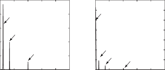
Next, we explore the in uence of a linear trend on a spectrum. Long-term

trends are common features in earth science data. We will see that this trend

is misinterpreted as a very long period by the FFT, producing a large peak

with a frequency close to zero (Fig. 5.7).

[Pxx,f] = periodogram(x,[],1024,1);

[Pxxt,f] = periodogram(xt,[],1024,1);

subplot(1,2,1)

plot(f,Pxx), grid

xlabel('Frequency')

122 5 TIME-SERIES ANALYSIS

Frequency

Power

=0.02

≈0.07

=0.2

=0.02

≈

0.07

=0.2

Linear trend

0.2

0.3

0.4

0.5

0.1

200

400

600

800

1000

2000

3000

4000

5000

6000

7000

0.2

0.3

0.4

0.5

0.1

Autospectrum

Fig. 5.7 Comparison of the auto-spectra for a the original noise-free signal with the periods

=50 (f

=0.02), τ

=15 (f

≈0.07) and τ

=5 (f

=0.2) and b the same signal overprinted on

a linear trend.  e linear trend is misinterpreted by the FFT as a very long period with a

high amplitude.

ylabel('Power')

subplot(1,2,2)

plot(f,Pxxt), grid

xlabel('Frequency')

ylabel('Power')

To eliminate the long-term trend, we use the function detrend.

xdt = detrend(xt);

subplot(2,1,1)

plot(t,x,'b-',t,xt,'r-'), grid

axis([0 200 -4 4])

subplot(2,1,2)

plot(t,x,'b-',t,xdt,'r-'), grid

axis([0 200 -4 4])

 e resulting spectrum no longer shows the low-frequency peak.

[Pxxt,f] = periodogram(xt,[],1024,1);

[Pxxdt,f] = periodogram(xdt,[],1024,1);

subplot(1,2,1)

plot(f,Pxx), grid

xlabel('Frequency')

ylabel('Power')

5.4 EXAMPLES OF AUTO-SPECTRAL AND CROSS-SPECTRAL ANALYSIS 123

5 TIME-SERIES ANALYSIS

Frequency

Power

Phase angle

=0.02

Corresponding phase

angle of 1.2568, equals

(1.2568*5)/(2*π)=1.001

012345

−2

−1

Crossspectrum

Phase Spectrum

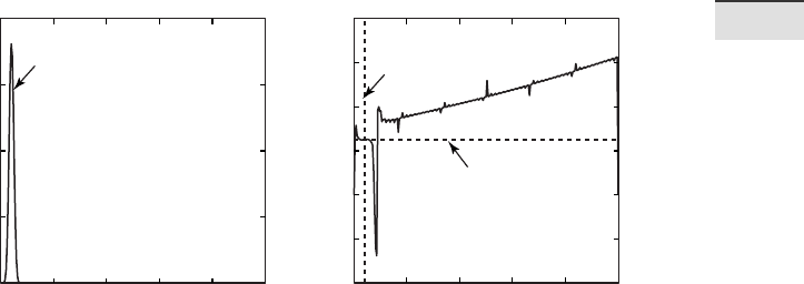
Fig. 5.8 Cross-spectrum of two sine waves with identical periodicities τ=5 (equivalent to

f=0.2) and amplitudes of 2.  e sine waves show a relative phase shi of t=1. In the argument

of the second sine wave this corresponds to 2π/5, which is one   h of the full wavelength

of τ=5. a  e magnitude shows the expected peak at f=0.2. b  e corresponding phase

di erence in radians at this frequency is 1.2566, which equals (1.2566*5)/(2*π)=1.0000,

which is the phase shi of 1 that we introduced at the beginning.

subplot(1,2,2)

plot(f,Pxxdt), grid

xlabel('Frequency')

ylabel('Power')

Some data contain a high-order trend that can be removed by  tting a high-

er-order polynomial to the data and by subtracting the corresponding x(t)

values.

We now use two sine waves with identical periodicities τ=5 (equivalent

to f=0.2) and amplitudes equal to two to compute the cross-spectrum of two

time series.  e sine waves show a relative phase shi of t=1. In the argu-

ment of the second sine wave this corresponds to 2π/5, which is one   h of

the full wavelength of τ=5.

clear

t = 1 : 1000;

x = 2*sin(2*pi*t/5);

y = 2*sin(2*pi*t/5 + 2*pi/5);

plot(t,x,'b-',t,y,'r-')

axis([0 50 -2 2]), grid

 e cross-spectrum is computed by using the function cpsd, which uses

Welch's method for computing power spectra (Fig. 5.8).

Pxy is complex and

124 5 TIME-SERIES ANALYSIS

contains both amplitude and phase information.

[Pxy,f] = cpsd(x,y,[],0,1024,1);

plot(f,abs(Pxy)), grid

xlabel('Frequency')

ylabel('Power')

title('Cross-Spectrum')

 e function cpsd(x,y,window,noverlap,nfft,fs) speci es the

number of FFT points

nfft used to calculate the cross power spectral den-

sity, which is 1024 in our example.  e parameter

window is empty in our

example, and therefore the default rectangular window is used to obtain

eight sections of

x and y.  e parameter noverlap de nes the number of

overlapping samples, which is zero in our example.  e sampling frequency

fs is 1 in this example.  e coherence of the two signals is one for all fre-

quencies since we are working with noise-free data.

[Cxy,f] = mscohere(x,y,[],0,1024,1);

plot(f,Cxy), grid

xlabel('Frequency')

ylabel('Coherence')

title('Coherence')

 e function mscohere(x,y,window,noverlap,nfft,fs) speci es

the number of FFT points

nfft=1024, the default rectangular window, and

the overlap of zero data points.  e complex part of

Pxy is required for com-

puting the phase shi between the two signals using the function

angle.

phase = angle(Pxy);

plot(f,phase), grid

xlabel('Frequency')

ylabel('Phase Angle')

title('Phase Spectrum')

 e phase shi at a frequency of f=0.2 (period τ=5) can be interpolated

from the phase spectrum

interp1(f,phase,0.2)

which produces the output

ans =

-1.2566

 e phase spectrum is normalized to one full period τ=2π, therefore the

phase shi of –1.2566 equals (–1.2566*5)/(2*π) = –1.0000, which is the phase

5.4 EXAMPLES OF AUTO-SPECTRAL AND CROSS-SPECTRAL ANALYSIS 125

5 TIME-SERIES ANALYSIS

shi of one that we introduced at the beginning.

We now use two sine waves with di erent periodicities to illustrate

cross-spectral analysis. Both signals

x and y have a periodicity of 5, but

with a phase shi of 1.

clear

t = 1 : 1000;

x = sin(2*pi*t/15) + 0.5*sin(2*pi*t/5);

y = 2*sin(2*pi*t/50) + 0.5*sin(2*pi*t/5+2*pi/5);

plot(t,x,'b-',t,y,'r-')

axis([0 100 -3 3]), grid

We can now compute the cross-spectrum Pxy, which clearly shows the

common period of τ=5 or frequency of f=0.2.

[Pxy,f] = cpsd(x,y,[],0,1024,1);

plot(f, abs(Pxy)), grid

xlabel('Frequency')

ylabel('Power')

title('Cross-Spectrum')

 e coherence shows a high value that is close to one at f=0.2.

[Cxy,f] = mscohere(x,y,[],0,1024,1);

plot(f,Cxy), grid

xlabel('Frequency')

ylabel('Coherence')

title('Coherence')

 e complex part of the cross-spectrum Pxy is required for calculating the

phase shi between the two sine waves.

[Pxy,f] = cpsd(x,y,[],0,1024,1);

phase = angle(Pxy);

plot(f,phase), grid

 e phase shi at a frequency of f=0.2 (period τ=5) is

interp1(f,phase,0.2)

which produces the output of

ans =

-1.2572

 e phase spectrum is normalized to one full period τ=2π, therefore the

126 5 TIME-SERIES ANALYSIS

phase shi of –1.2572 equals (–1.2572*5)/(2*π) = –1.0004, which is again

the phase shi of one that we introduced at the beginning.

5.5 Interpolating and Analyzing Unevenly-Spaced Data

We can now use our experience in analyzing evenly-spaced data to run a

spectral analysis on unevenly-spaced data. Such data are very common in

earth sciences, for example in the  eld of paleoceanography, where deep-

sea cores are typically sampled at constant depth intervals.  e transforma-

tion of evenly-spaced length-parameter data to time-parameter data in an

environment with changing length-time ratios results in unevenly-spaced

time series. Numerous methods exist for interpolating unevenly-spaced se-

quences of data or time series.  e aim of these interpolation techniques for

x(t) data is to estimate the x-values for an equally-spaced t vector from the

irregularly-spaced x(t) actual measurements. Linear interpolation predicts

the x-values by e ectively drawing a straight line between two neighboring

measurements and by calculating the x-value at the appropriate point along

that line. However, this method has its limitations. It assumes linear transi-

tions in the data, which introduces a number of artifacts, including the loss

of high-frequency components of the signal and the limiting of the data

range to that of the original measurements.

Cubic-spline interpolation is another method for interpolating data that

are unevenly spaced. Cubic splines are piecewise continuous curves, requir-

ing at least four data points for each step.  e method has the advantage that

it preserves the high-frequency information contained in the data. However,

steep gradients in the data sequence, which typically occur adjacent to ex-

treme minima and maxima, could cause spurious amplitudes in the inter-

polated time series. Since all these and other interpolation techniques might

introduce artifacts into the data, it is always advisable to (1) keep the total

number of data points constant before and a er interpolation, (2) report

the method employed for estimating the evenly-spaced data sequence, and

(3) explore the e ect of interpolation on the variance of the data.

Following this brief introduction to interpolation techniques, we can

apply the most popular linear and cubic spline interpolation techniques

to unevenly-spaced data. Having interpolated the data, we can then use

the spectral tools that have previously been applied to evenly-spaced data

(Sections 5.3 and 5.4). We must  rst load the two time series:

clear

series1 = load('series1.txt');

5.5 INTERPOLATING AND ANALYZING UNEVENLY-SPACED DATA 127

5 TIME-SERIES ANALYSIS

series2 = load('series2.txt');

Both synthetic data sets contain a two-column matrix with 339 rows.  e

 rst column contains ages in kiloyears, which are unevenly spaced.  e sec-

ond column contains oxygen-isotope values measured on calcareous algae

(foraminifera).  e data sets contain 100, 40 and 20 kyr cyclicities and they

are overlain by Gaussian noise. In the 100 kyr frequency band, the second

data series has shi ed by 5 kyrs with respect to the  rst data series. To plot

the data we type

plot(series1(:,1),series1(:,2))

figure

plot(series2(:,1),series2(:,2))

 e statistics for the spacing of the  rst data series can be computed by

intv1 = diff(series1(:,1));

plot(intv1)

 e plot shows that the spacing varies around a mean interval of 3 kyrs with

a standard deviation of ca. 1 kyrs.  e minimum and maximum values for

the time axis

min(series1(:,1))

max(series1(:,1))

of t

min

=0 and t

max

=997 kyrs provide some information about the tempo-

ral range of the data.  e second data series

intv2 = diff(series2(:,1));

plot(intv2)

min(series2(:,1))

max(series2(:,1))

has a similar range from 0 to 997 kyrs. We see that both series have a mean

spacing of 3 kyrs and range from 0 to ca. 1000 kyrs. We now interpolate the

data to an evenly-spaced time axis. While doing this, we follow the rule that

the number of data points should not be increased.  e new time axis runs

from 0 to 996 kyrs with 3 kyr intervals.

t = 0 : 3 : 996;

We can now interpolate the two time series to this axis with linear and

spline interpolation methods, using the function

interp1.

series1L = interp1(series1(:,1),series1(:,2),t,'linear');