Velten K. Mathematical Modeling and Simulation: Introduction for Scientists and Engineers
Подождите немного. Документ загружается.


3.10 More Examples 205
data characterizing your system. Then, the parameter estimation procedures
described in this section (and the underlying regression techniques described in
Chapter 2) can often be used to estimate the parameter from the available data.
3.10
More Examples
ODEs can be applied in many, if not in most situations where your data describe the
evolution of a quantity of interest over time. The following examples are intended
to give you an idea of the wide applicability of this method. They will also be used
to explain some useful concepts beyond the theory discussed above, such as the
discussion of ideas of the theory of dynamical systems in Section 3.10.1 or of the
concept of compartmental modeling in Section 3.10.3.
3.10.1
Predator–Prey Interaction
Population sizes of animals often have an oscillatory nature, that is, they increase
and decrease periodically over time. In some cases, this can be explained by
predator–prey interactions. Consider two animal species, a predator species and a
prey species serving as the food of the predator. Let x and y denote their respective
population sizes, measured, for example, as the number of species per square
kilometer. If the prey population x is sufficiently large, the predator population y
will increase since there is enough food available. The increase in the predator
population y, however, will decrease the prey population x until the predator
population finally runs short of food. Hence, the decrease in the prey population
x will be followed by a decrease in the predator population y ,untily is reduced
so much that the prey population x increases again, which will be followed by a
subsequent increase in y,andsoon.Ifyousketchx and y in this way, you will find
that one can expect periodical curves having the same period length, but a little bit
shifted in time, that is, the maximum of x being followed by the maximum of y
some time later.
3.10.1.1 Lotka–Volterra Model
In 1926, Volterra investigated fish population data exhibiting this kind of dynamics,
and he used the following model to explain the data [114–116]:
x
(t) = (r − ay(t)) · x(t) (3.269)
y
(t) = (bx(t) − m) · y(t) (3.270)
In these equations, a, r, b and m are parameters (real constants) that are discussed
below. Since the equations were independently found by Lotka and Volterra [115,
117], they are known as the Lotka–Volterra model.

206 3 Mechanistic Models I: ODEs
To understand this model, let us consider some special cases. In the absence of
the predator (y = 0), we have
x
(t) = r · x(t) (3.271)
Using the methods of Section 3.7, you can easily show that this is solved by
x (t) = x
0
· e
rt
(3.272)
where x
0
= x(0). Hence, the above model assumes an exponential increase in the
prey population in the absence of the prey. Applying the same reasoning to the case
x = 0, you find that the model assumes an exponential decrease in the predator
population in the absence of preys:
y(t) = y
0
· e
−mt
(3.273)
where y
0
= y(0). Particularly, the exponential increase in the prey population is
certainly a wrong assumption if the prey population becomes large enough. But
this is irrelevant here since the model refers to the situation y = 0 where the prey
population is limited by the presence of the predator. The growth rates r and m in
Equations 3.269 and 3.270 can be interpreted similar to the interpretation of the
parameter r of the body temperature model in Section 3.4.1.2:
•
r, the growth rate of the prey, expresses the percent increase
of x per unit of time, expressed relative to the actual size of x;
a typical unit would be day
−1
•
m, the death rate of the predator, expresses the percent
decrease of y per unit of time, expressed relative to the actual
size of y;again,atypicalunitwouldbeday
−1
Equations 3.269 and 3.270 show that the growth rate of the prey population
is assumed to be reduced proportionally to the size of the predator population,
while the death rate of the predator is reduced proportionally to the size of the
prey population. This is governed by the parameters a and b with the following
interpretations:
•
a expresses the decrease in the growth rate of the prey per
unit of y;atypicalunitwouldbeday
−1
•
b expresses the increase in the growth rate of the predator
per unit of x; a typical unit would be day
−1
A closed form solution of Equations 3.269 and 3.270 cannot be obtained (try
it ...), although one can at least derive an implicit equation characterizing the
solution, see [114, 116]. Figure 3.15a shows an example where Equations 3.269 and
3.270 have been solved numerically using the R program
Volterra.r in the book
software.
Volterra.r has been obtained by an appropriate editing of ODEEx2.r
3.10 More Examples 207
020
50
100
x, y
u, v
150
40 60
t
80 100
0 204060
t
(a)
(b)
80 100
0.8
1.0
1.2
1.4
1.6
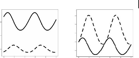
Fig. 3.15 (a) Prey (line) and predator (dashed line) popu-
lation sizes obtained using
Volterra.r and r = 0.1, m =
0.15, a = 0.002, b = 0.001, x
0
= 170, and y
0
= 40. (b) Same
plot in nondimensional form obtained using
VolterraND.r
and ˜r = 0.1, ˜m = 0.15,
˜
a = 0.08,
˜
b = 0.17, u
0
= 1, and
v
0
= 1.
(Section 3.8.3.7). Note that the curves in Figure 3.15a follow exactly that ‘‘shifted’’
periodical pattern that has been conjectured above.
3.10.1.2 General Dynamical Behavior
As it was said above, Volterra found the ODE system Equations 3.269 and 3.270
when he tried to understand certain oscillatory fish population data. He found a
good coincidence between these ODEs and his data, and one could say that in this
way these ODEs did what they where expected to do. But it is in fact a big advantage
of mathematical modeling using ODEs that this is not necessarily the endpoint of
the analysis. When a good coincidence between an ODE and data is found, we have
a good reason to believe that these ODEs capture essential aspects governing the
dynamics of the system. Then it makes sense to perform a theoretical investigation
of the general dynamical behavior of the ODE system, that is, of the behavior of
the system for all kinds of initial and parameter values, because in this way we
may hope to learn about the general dynamical behavior of the real system that
produced the data. For example, if we are investigating fish population data such
as Volterra, we may be interested to learn about conditions that would increase the
population size of a particular fish species beyond some acceptable level.
An analysis of the general dynamical behavior of an ODE system can be performed
based on the theory of dynamical systems, which provides methods to understand
and classify the patterns of dynamical behavior that solutions of ODE systems may
have. An extensive discussion of these methods is beyond the scope of this book.
You may find a detailed analysis of the dynamical behavior of the Lotka–Volterra
model in [114, 116]. We will confine ourselves here to a discussion of two aspects of
the analysis of the dynamical behavior of ODEs, which is something like a minimal
knowledge you should have of this kind of analysis: the formulation of an ODE (or
PDE) in dimensionless form and the phase plane plot.
208 3 Mechanistic Models I: ODEs
3.10.1.3 Nondimensionalization
As to the first of these points, note that exactly the same picture as in Figure 3.15a
would have been obtained using, for example, x
0
= 1700 and y
0
= 400 together
with an appropriate scaling of the other parameters of the model. This means that
if we want to classify the dynamical behavior of an ODE, we should first try to get
rid of these scaling issues that just change the numbers at the axes of our plots, but
that do not affect the qualitative dynamical behavior of the solution. This is done
by bringing the ODE in dimensionless form. Referring to Equations 3.269 and 3.270,
thiscanbedoneasfollows.Letx
r
, y
r
,andt
r
be reference values of x, y ,andt (the
appropriate choice of these values is discussed below). Now define u, v,andτ as
follows:
u =
x
x
r
(3.274)
v =
y
y
r
(3.275)
τ =
t
t
r
(3.276)
All quantities defined in these equations are dimensionless since they are all
expressed as fractions involving two quantities having the same dimensions. Since
dimensions enter Equations 3.269 and 3.270 only through x, y,andt,wegetridof
all dimensions in these equations if we substitute u, v,andτ into these equations
using Equations 3.274–3.276. The result is
du
dτ
= (rt
r
− at
r
y
r
v)u (3.277)
dv
dτ
= (bt
r
x
r
u − mt
r
)v (3.278)
or
du
dτ
= (
˜
r −
˜
av)u (3.279)
dv
dτ
= (
˜
bu −
˜
m)v (3.280)
using the identifications
˜
r = rt
r
,
˜
a = at
r
y
r
,
˜
b = bt
r
x
r
,and
˜
m = mt
r
. Note that the
structure of the last two equations is identical with the structure of Equations 3.269
and 3.270, and that all quantities appearing in Equations 3.279 and 3.280 are indeed
dimensionless (verify this for
˜
r,
˜
a,
˜
b,
˜
m).
Now it is time to talk about the proper choice of the reference values x
r
, y
r
,andt
r
in Equations 3.274–3.276. Principally, these quantities can be chosen arbitrarily.
In some cases, your application may suggest ‘‘natural’’ reference values that can
be used. t
r
is usually set to the appropriate unit of time corresponding to the time
scale on which the state variables of the ODE are observed, which means that
you would set t
r
= 1 day (or week, or year) in most models involving population
dynamics. In the absence of other ‘‘natural’’ reference values, the reference values
3.10 More Examples 209
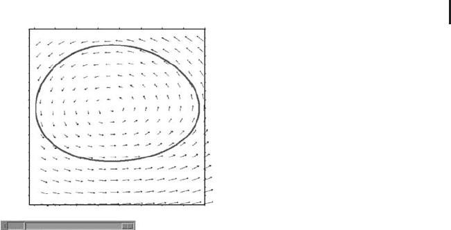
v
u
r
0.0999
1.5
1.25
1
0.75
0.7 0.8 0.9 1 1.1
Fig. 3.16 Phase plot of the result in Figure 3.15b, generated
using
VolPhase.mac.Thelineisthecurve(u(t), v(t)) and
the arrows show the vector field (du/dτ , dv/dτ ). Note the
slider below that can be used to change the value of r inter-
actively.
for the state variables of the ODE are often set to the initial values of the ODE,
which corresponds to x
r
= x
0
and y
r
= y
0
in our case.
Figure 3.15b shows the solution of Equations 3.279 and 3.280 using parameter
values exactly corresponding to those used in Figure 3.15a. This figure was
obtained using
VolterraND.r in the book software. In contrast to Figure 3.15a,
the axes in Figure 3.15b are in dimensionless units, which means that Figure 3.15b
summarizes the dynamical behavior of the ODE for a great number of different
situations. For example, depending on your setting of t
r
,thevaluesonthet axis
may refer to seconds, days, years, and so on. In the same way, the values on the
u, v axis may refer to the number of individuals, but they may also refer to any
other units which you choose by setting x
r
and y
r
. Analyzing ODEs in this way
it is much easier to get a picture of its overall dynamical behavior. See Murray
[114] for a more detailed analysis of the dynamical behavior of the Lotka–Volterra
equations. After introducing natural choices of the reference values x
r
, y
r
and t
r
,
Murray reduces Equations 3.279 and 3.280 to a form which involves only one
parameter. An analysis of this system shows, for example, that the Lotka–Volterra
equations are structurally instable in the sense that for certain initial conditions,
small perturbations of these initial conditions or parameters can have large effects
on the solution, which limits the practical usefulness of this model as discussed
in [114].
3.10.1.4 Phase Plane Plots
For systems of two ODEs, the solution can also be plotted in a phase plane plot,
which is particularly useful for an understanding of the overall dynamical behavior
of the ODEs. Figure 3.16 shows a phase plane plot of the solution of Equations
3.279 and 3.280 using exactly the same parameters as in Figure 3.15b. In the phase
plane plot, the coordinate axes correspond to the state variables u and v,andthereis

210 3 Mechanistic Models I: ODEs
no time axis. This means that what you see in the phase plot is the curve (u(t), v(t)),
drawnonsomeinterval[t
0
, t
1
]. Comparing Figures 3.16 and 3.15b you will find
that both figures indeed refer to the same solution of Equations 3.279 and 3.280.
Figure 3.16 has been produced using the Maxima program
VolPhase.mac.With
some effort, R could also have been used to produce similar plots, but Maxima
provides a really nice package called
plotdf to produce phase plots that has been
used in
VolPhase.mac. The command producing the phase plot in this program is
1: plotdf(
2: [(r-a*v)*u,(b*u-m)*v]
3: ,[u,v]
4: ,[parameters, "r=0.1,m=0.15,a=0.08,b=0.17"]
5: ,[sliders,"r=0.07:0.1"]
6: ,[trajectory_at,1,1]
7: ,[tstep,0.1]
8: ,[nsteps,1000]
9: ,[u,0.69,1.1]
10: ,[v,0.7,1.7]
11: )$
(3.281)
In this code, line 2 defines the ODEs (3.279) and (3.280) via their right-hand sides.
The rest of the code is self-explanatory. Note the definition of the slider element
in line 5, which can be used to change the parameter value of r interactively
(Figure 3.16). Several of such parameter sliders can be added to the plot in this way.
Lines 7–8 define the interval [0, T]forwhichthecurve(u(t), v(t)) is plotted. We have
T =
tstep · nsteps here which gives T = 100 based on the settings in 3.281, and
this means that Figure 3.16 uses the same time interval as Figure 3.15b.
tstep
is the stepsize of the numerical algorithm. plotdf uses the Adams–Moulton
method, but it can also be switched to a Runge–Kutta method (Section 3.8) with
an adaptive stepsize [110]. If you use
plotdf as above, you should choose tstep
small enough, applying the heuristical procedures explained in Section 3.8 (Note
3.8.1).
The closed form of the trajectory in Figure 3.16 expresses the fact that the curve
(u(t), v(t )) always goes along the same way, which means that this is indeed a
periodical solution. It would not have been so easy to see this in the conventional
plot, Figure 3.15b. The real benefit of the phase plot, however, lies in the fact that
you can see the effects of changes of the initial conditions or of the parameters. If you
move the parameter slider in Figure 3.16, you can see that the trajectory changes its
size and position, and you can assess in this way the effects of parameter changes
much better than it would have been possible using conventional plots such as
Figure 3.15b. Try this yourself using
VolPhase.mac. Effects of different initial
condition can be studied particularly simple just by clicking into the plot. Every click
produces a trajectory going through the initial condition at your mouse position.
An example is shown in Figure 3.17a. This figure shows an interesting fact: you
see that the amplitudes of the oscillations of the predator and prey populations go
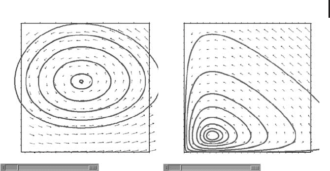
3.10 More Examples 211
v
u
r
0.0999
1.5
1.25
1
0.75
0.7 0.8 0.9 1 1.1
v
u
r
0.0999
10
7.5
5
2.5
0123
(a) (b)
Fig. 3.17 (a) Phase plot as in Figure 3.16, including several
other phase trajectories for different initial conditions. (b)
Phase plot as in (a) but based on a different scaling, show-
ing the instability of the Lotka–Volterra equations.
to zero as you approach a point in the center of the smallest, inner curve. This
corresponds to a singular point of the ODEs, see the discussion in [114].
Figure 3.17b shows a similar plot using a different scaling of the axes, and a
number of trajectories with initial conditions approaching the coordinate axes.
This figure shows the structural instability of the Lotka–Volterra equations that was
mentioned above (for a detailed analysis we refer to [114]): imagine you have initial
conditions somewhere below the singular point infinitesimally close to the u axis
of the plot, and imagine an infinitesimal perturbation of these initial conditions,
which puts you on one of the neighboring trajectories. Then, comparing this
neighboring trajectory with your original trajectory, you will find that you have
large (i.e. noninfinitesimal) differences between these trajectories in regions of the
phase space far away from the coordinate axes, as it can be seen in Figure 3.17b.
3.10.2
Wine Fermentation
Grape juice is transformed into wine in the fermentation process. This is a
very complex process which is still not fully understood, and which involves the
metabolization of sugar into ethanol by yeast cells [118, 119]. Loosely speaking,
one can say the yeast in the fermenter ‘‘eats up’’ the sugar and excretes ethanol. If
everything works well, the yeast cells will utilize most of the sugar in the fermenter
during 7–10 days [120, 121]. It may happen, however, that the fermentation needs a
much longer time (sluggish fermentation) or the fermentation may even stop before
a sufficient amount of sugar is metabolized by the yeast cells (stuck fermentation). In
an industrial setting, this kind of abnormalities can be very expensive, for example,
in terms of extended processing times in the case of sluggish fermentations or in

212 3 Mechanistic Models I: ODEs
terms of microbial instabilities in the case of stuck fermentations that endanger
the quality of the final product. This leads to the following problem:
Problem 1:
How can the fermentation process be controlled in a way that avoids sluggish or
stuck fermentations?
3.10.2.1 Setting Up a Mathematical Model
To address this problem, the process engineer can try to tune a number of variables
that have an impact on the way in which the fermentation proceeds. One of these
control parameters is the nitrogen concentration in the fermenter which we denote
N(t)(gl
−1
), where t is time (h
−1
). Nitrogen is an important nutrient needed by the
yeast cells (too low nitrogen levels can be a limiting factor of yeast cell growth).
N(t) refers to the total yeast available nitrogen concentration and includes various
subtypes which we do not need to discuss here [121]. Another important control
variable that is discussed here is the temperature T(t)(K).Consideringthesetwo
control variables, the process engineer has to answer the following question:
Q: How should N(t)andT(t) be adjusted during fermentation in order to avoid
sluggish or stuck fermentations?
Referring to the definition of mathematical models as a triple (S, Q, M) consisting
of a system S,aquestionQ and a set of mathematical statements M (Definition
1.4.1), this is the question we are going to ask here, and obviously S can be
identified with the fermenter. What remains to be done is the formulation of the
set of mathematical statements, M, which will be a system of ODEs. The above
question Q tells us that N(t)andT(t) will be variables of our mathematical model,
and since the question focuses on sluggish or stuck fermentations, it is obvious that
we will also need to compute the sugar concentration S(t)[gl
−1
). You can see here
that the question Q we are asking is a really essential ingredient of a mathematical
model that guides the formulation of the mathematical equations. Since we have
said that the yeast cells ‘‘eat up’’ the sugar, it is obvious that we will not be able to
compute the dynamics of S(t)unlesswehaveavariableexpressingthe(viable)yeast
cell concentration. Let us denote this as X(t) (gram biomass per liter). Now we have
to formulate equations for these variables. In the modeling and simulation scheme
(Note 1.2.3), this is at the heart of the systems analysis step, and this is the point
where we have to refer to appropriate specialized literature. In this case, any book
on fermentation technology can be used, which describes the processes that are
involved in the metabolization of sugar and nitrogen into ethanol by the yeast cells
[118, 119]. The result of such an analysis as well as a lot of background regarding
the equations we are going to write now can be found in a model formulated by
Blank [122]. Blank’s model is an improved version of the fermentation model of
Cramer et al. [121].

3.10 More Examples 213
Table 3.3
Statevariablesofthewinefermentationmodel.
State variable Description Unit
X (Viable) yeast cell concentration gram biomass per liter
N (Yeast available) nitrogen concentration gram nitrogen per liter
E Ethanol concentration gram ethanol per liter
S Sugar concentration gram sugar per liter
3.10.2.2 Yeast
Regarding X(t), Cramer et al. use the following balance equation:
dX
dt
= μ · X − k
d
· X (3.282)
This means that the yeast cells grow proportionally to the actual yeast cell
concentration X, the proportionality constant being the specific growth rate μ.
At the same time, the yeast cells are inactivated or die proportionally to X,
the proportionality constant being the death constant k
d
. Note that you find
all information regarding the state variables and parameters discussed here in
Tables 3.3 and 3.4. If μ and k
d
would be just constants, Equation 3.282 could be
written as
dX
dt
=˜μ · X (3.283)
with ˜μ = μ − k
d
, which means that X(t) would follow a simple exponential growth
pattern. In reality, however, μ and k
d
depend on a number of factors, and these
dependencies must be described based on appropriate empirical data. In fact,
the final predictive power of a fermentation model depends very much on the
appropriate description of these empirical dependencies. Regarding μ,Cramer
[121] uses the following expression:
μ = μ
max
·
N
K
N
+ N
(3.284)
This means that the growth of the yeast cells is limited by nitrogen availability. The
algebraic form of the right-hand side of this equation is frequently used to describe
the rate of enzyme-mediated reactions, and it is known as the Michaelis–Menten ki-
netics term. Assuming a maximum rate V
max
for some particular enzyme-mediated
reaction and denoting the actual reaction rate and the substrate concentration with
V and C, respectively, the Michaelis–Menten kinetics is usually written as
V = V
max
·
C
K
m
+ C
(3.285)

214 3 Mechanistic Models I: ODEs
Table 3.4 Parameters of the wine fermentation model.
Parameter Description Unit Value Source
μ Specific growth rate h
−1
(3.284) [121]
μ
max
Maximum specific
growth rate
h
−1
(3.286) [122, 124, 125]
T Temperature K Data [122]
K
N
Monod constant for
nitrogen
g nitrogen/l 0.01 [121]
k
d
Death constant h
−1
(3.287) [121]
k Specific death constant l/g ethanol//h Unknown
Y
XN
Stoichiometric yield
coefficient of biomass on
nitrogen
g biomass/g
nitrogen
18 [127]
β Specific ethanol
production rate
gethanol/g
biomass/h
(3.289) [121]
β
max
Maximum specific
ethanol production rate
gethanol/g
biomass/h
(3.290) [121,126]
β
max,24
◦
C
Maximum specific
ethanol production rate
at 24
◦
C
gethanol/g
biomass/h
0.3 [121]
K
S
Michaelis–Menten-type
constant for sugar
g sugar/l 10 [121]
Y
ES
Stoichiometric yield
coefficient of ethanol on
sugar
gethanol/g
sugar
0.47 [121]
X
0
Initial yeast
concentration at t = 0
g biomass/l 0.2 fermentation.csv
E
0
Initial ethanol
concentration at t = 0
gethanol/l 0 fermentation.csv
S
0
Initial sugar
concentration at t = 0
g sugar/l 205 fermentation.csv
N
0
Initial nitrogen
concentration at t = 0
g nitrogen/l Unknown
N
i
add
ith nitrogen addition
(i = 1, ..., n)
g nitrogen/l 0.03 (i = 1,2) [122]
t
i
add
Time of ith nitrogen
addition (i = 1, ..., n)
h 130 (i = 1),
181 (i = 2)
[122]
where K
m
is the Michaelis–Menten constant which corresponds to the substrate
concentration that generates V
max
/2 [123]. It can be easily derived from Equation
3.285 that V → V
max
as C →∞.
Applying this to Equation 3.284, you see that μ
max
is the maximum specific
growth rate, and that μ approaches this maximum growth rate asymptotically as
the available amount of nitrogen increases. The Michaelis–Menten constant K
N
expresses the nitrogen concentration which corresponds to μ = μ
max
/2. Note that