Velten K. Mathematical Modeling and Simulation: Introduction for Scientists and Engineers

Подождите немного. Документ загружается.

4.2 The Heat Equation 235

Fourier’s law can also be written as

q =−K ·∇T (4.6)

In these equations, q is the heat ﬂow rate (W m

−2

). In a situation where you do

not have temperature gradients in the y and z directions (such as Problem 1 in

Section 4.1.3), Fourier’s law attains the one-dimensional form

=−K ·

(4.7)

So, you see that Fourier’s law expresses a very simple proportionality: the heat

ﬂow in the positive x direction is negatively proportional to the temperature

gradient. This means that a temperature which is going down in the positive x

direction (corresponding to a negative value of dT/dx) generates a heat ﬂow in

the positive x direction. This expresses our everyday experience that heat ﬂows are

always directed from higher to lower temperatures (e.g. from your hot coffee cup

toward its surroundings).

4.2.2

Conservation of Energy

Let us now try to understand the heat equation. Remember that in the ODE models

discussed in Chapter 3, the left-hand sides of the ODEs usually expressed rates

of changes of the state variables, which were then expressed in the right-hand

sides of the equations. Take the body temperature model as an example: as

was explained in Section 3.4.1, Equation 3.28 is in an immediate and obvious

correspondence with a statement describing the temperature adaption such as the

sensor temperature changes proportionally to the difference between body temperature and

actual sensor temperature. Regarding PDEs, the correspondence with the process

under consideration is usually not so obvious. If you are concerned with PDEs

for some time, you will of course learn to ‘‘read’’ and understand PDEs and

their correspondence with the processes under consideration to some extent,

but understanding a PDE still needs one or two thoughts more as compared to

ODEs. Equation 4.1, for example, involves a combination of ﬁrst- and second-order

derivatives with respect to different variables which expresses more than just a rate

of change of a quantity as was the case with ODEs. The problem is that PDEs

simultaneously express rates of changes of several quantities.

Fourier’s law provides us with a good starting point for the derivation of Equation

4.1. It is in fact one of the two main ingredients in the heat equation. What could

the other essential ingredient possibly be? From the ODE point of view, we could

say that Fourier’s law expresses the consequences of rates of changes of the

temperature with respect to the spatial variables x, y,andz. So, it seems obvious

that we have to look for equations expressing the rate of change of temperature

with respect to the remaining variable, which is time t.Suchanequationcanbe

derived from the conservation of energy principle [145].

236 4 Mechanistic Models II: PDEs

01x

x + Δx

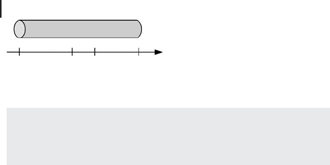
Fig. 4.2 Interval [x, x + x] corresponding to a small part of a one-dimensional body.

Note 4.2.1 (Deriving PDEs using conservation principles) Many of the impor-

tant PDEs of mathematical physics can be derived from conservation principles

such as conservation of energy, conservation of mass,orconservation of momentum

(see the examples in Section 4.10).

The most intuitive and least technical way to apply energy conservation is the

consideration of a small interval [x, x + x] corresponding to a small part of a

one-dimensional body (Figure 4.2).

Remember from your physics courses that the energy conservation principle

states that energy cannot be created or destroyed, which means that the total

amount of energy in any closed system remains constant. Applied to [x, x + x]

(you should always think of the part of the physical body corresponding to

[x, x + x] when we write down this interval in the following) this means that

any change in the energy content of [x, x + x] must equal the amount of heat

that ﬂows into [x, x + x] through its ends at x and x + x. Note that there can

be no ﬂow in the y and z directions since we assume a one-dimensional body

here. For example, imagine the outer surface of the cylinder in Figure 4.2 to be

perfectly insulated against heat ﬂow (see Section 4.3.3 for more on dimensionality

considerations). The heat balance of [x, x + x] can be written as

⎧

⎪

⎨

⎪

⎩

Rate of change

of energy content

in [x, x + x]

⎫

⎪

⎬

⎪

⎭



Netheatinﬂow

through x and x + x

(4.8)

4.2.3

Heat Equation = Fourier’s Law + Energy Conservation

Basically, the heat equation can now be derived by putting together the results of the

last two sections. To this end, consider some small time interval [t, t + t]. Within

this time interval, the temperature at x will change from T(x, t)toT(x, t + t). This

corresponds to a change in the energy content of [x, x + x]thatwearegoingto

estimate now. First of all, note that for sufﬁciently small x,wehave

x, t) ≈ T(x, t) ∀

x ∈ [x, x + x] (4.9)

4.2 The Heat Equation 237

and

x , t + t) ≈ T(x, t + t) ∀

x ∈ [x, x + x] (4.10)

The last two equations say that we may take T(x, t)toT(x, t + t) as the ‘‘rep-

resentative temperatures’’ in [x, x + x]attimest and t + t, respectively. This

means that we are now approximately in the following situation: we have a physical

body corresponding to [x, x + x], which changes its temperature from T(x, t)to

T(x, t + t). Using the above explanation of C and denoting the mass of [x, x + x]

with m,we,thus,have

⎧

⎪

⎨

⎪

⎩

Rate of change

of energy content

in [x, x + x]

⎫

⎪

⎬

⎪

⎭

= C · m · (T(x, t + t) −T(x, t)) (4.11)

Denoting the cross-sectional area of the body in Figure 4.2 with A,wehave

m = Axρ, which turns Equation (4.11) into

⎧

⎪

⎨

⎪

⎩

Rate of change

of energy content

in [x, x + x]

⎫

⎪

⎬

⎪

⎭

= C · Axρ · (T(x, t + t) − T(x, t)) (4.12)

This gives us the left-hand side of Equation 4.8. The right-hand side of this

equation can be expressed as



Netheatinﬂow

through x and x + x

= At(q

(x) − q

(x + x)) (4.13)

using the heat ﬂow rate q

introduced above. Note that the multiplication with At

is necessary in the last formula since q

expresses heat ﬂow per units of time and

surface area: its unit is (W m

−2

) = (J s

−1

−2

). Note also that the signs used in the

difference q

(x) − q

(x + x) are chosen such that we get the net heat inﬂow as

required. Using Equations 4.8, 4.12, and 4.13, we obtain the following:

T(x, t + t) − T(x, t)

t

Cρ

(x) − q

(x + x)

x

(4.14)

Using Fourier’s law, Equation 4.7 gives

T(x, t + t) − T(x, t)

t

Cρ

∂T(x + x, t, t)

∂x

−

∂T(x, t)

∂x

x

(4.15)

From this, the heat equation (4.1) is obtained by taking the limit for t → 0and

x → 0.

238 4 Mechanistic Models II: PDEs

4.2.4

Heat Equation in Multidimensions

The above derivation of the heat equation can be easily generalized to multidimen-

sions by expressing energy conservation in volumes such as [x, x + x] × [y, y +

y]. Another option is to use an integral formulation of energy conservation over

generally shaped volumes, which leads to the heat equation by an application of

standard integral theorems [101]. In any case, the ‘‘small volumes’’ that are used to

consider balances of conserved quantities such as energy, mass, momentum, and

so on, similar to above are usually called control volumes. Beyond this, you should

note that the parameters C , ρ,andK may depend on the space variables. Just

check that the above derivation works without problems in the case where C and ρ

depend on x.IfK depends on x, the above derivation gives

∂T(x, t)

∂t

Cρ

∂

∂x



K(x) ·

∂T(x, t)

∂x



(4.16)

instead of Equation 4.1 and

∂T(x, t)

∂t

Cρ



∂

∂x



K(x) ·

∂T(x, t)

∂x



∂

∂x



K(x) ·

∂T(x, t)

∂x



∂

∂x



K(x) ·

∂T(x, t)

∂x



(4.17)

inthecasewhereK depends on the space coordinates x = (x

, x

)

.Usingthe

nabla operator ∇ (Equation 4.5), the last equation can be written more compactly as

∂T(x, t)

∂t

Cρ

∇



K(x) ·∇T(x, t)



(4.18)

4.2.5

Anisotropic Case

Until now, the thermal conductivity was assumed to be independent of the direction

of measurement. Consider a situation with identical temperature gradients in the

three main space directions, that is,

∂T

(4.19)

Then, Fourier’s law (Equation 4.6) says that

= K ·

∂T

= q

= K ·

∂T

= q

= K ·

∂T

(4.20)

that is, the heat ﬂux generated by the above temperature gradients is independent

of the direction in space (note that this argument can be generalized to arbitrary

4.2 The Heat Equation 239

directions). A material with a thermal conductivity that is direction independent

in this sense is called isotropic. The term ‘‘isotropy’’ is used for other material

properties such as ﬂuid ﬂow permeability or electrical conductivity in a similar way.

Materials that do not satisfy the isotropy condition of directional independence are

called anisotropic. For example, an anisotropic material may have a high thermal

conductivity in the x

direction and smaller conductivities in the other space

directions. A single number K obviously does not sufﬁce to describe the thermal

conductivity in such a situation, which means you need a multi- or matrix-valued

thermal conductivity K such as

K =

⎛

⎜

⎝

⎞

⎟

⎠

(4.21)

Many other anisotropic material properties are described using matrices or

tensors in a similar way, while isotropic material properties are described using

a single scalar quantity such as the scalar thermal conductivity in Fourier’s law

(Equation 4.6) above. Thanks to matrix algebra, Equation 4.6 and the heat equation

(4.18) remain almost unchanged when we use K from Equation 4.21:

q(x, t) =−K ·∇T(x, t) (4.22)

∂T(x, t)

∂t

Cρ

∇



K(x) ·∇T(x, t)



(4.23)

The diagonal entries of K describe the thermal conductivities in the main space

directions, that is, K

is the thermal conductivity in x

direction, K

in x

direction,

and so on.

4.2.6

Understanding Off-diagonal Conductivities

To understand the off-diagonal entries, consider the following special case:

K =

⎛

⎜

⎝

0 K

00K

⎞

⎟

⎠

(4.24)

Applying this in Equation 4.22, the heat ﬂow in the x

direction is obtained as

follows:

(x, t) = K

∂T(x, t)

∂x

+ K

∂T(x, t)

∂x

(4.25)

So, you see that K

= 0 means that the heat ﬂow in the x

direction depends

not only on the temperature gradient in that direction, ∂T/∂x

,butalsoonthe

temperature gradient in the x

direction, ∂T/∂x

. You may wonder how this is

240 4 Mechanistic Models II: PDEs

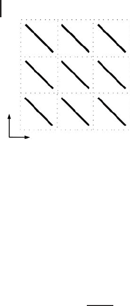
Fig. 4.3 Periodicity cells of a medium with an anisotropic effective thermal conductivity.

possible, so let us consider an example. Figure 4.3 shows a ‘‘microscopic picture’’

of a periodic medium in the x

plane. Here, ‘‘periodic medium’’ means that the

medium is assumed to consist of a great number of periodicity cells such as those

shown in the ﬁgure. ‘‘Microscopic picture’’ is to say that the ﬁgure just shows a

few of the periodicity cells, which we assume to be very small parts of the overall

geometry of the medium in the x

plane (we do not need the overall geometry

for our argument). Now assume that the black bars in the medium consist of

a material having zero thermal conductivity, while the matrix surrounding the

bars has some ﬁnite (scalar) thermal conductivity. If we now apply a temperature

gradient in the x

direction, this will initiate a heat ﬂow in the same direction:

(x, t) = K

∂T(x, t)

∂x

(4.26)

Here, K

denotes the (isotropic) thermal conductivity of the matrix surrounding

the black bars in Figure 4.3. But due to the heat-impermeable bars in the medium,

this heat ﬂow cannot go straight through the medium in the x

direction. Rather,

it will be partially deﬂected into the x

direction by the action of the bars. In this

way, a temperature gradient in the x

direction can indeed initiate a heat ﬂow in

the x

direction. If one then assumes the periodicity cells in Figure 4.3 to be very

small in relation to the overall size of the medium and derives ‘‘effective’’, averaged

thermal conductivities for the medium, one arrives at thermal conductivity matrices

with off-diagonal entries similar to Equation 4.24. Such effective (‘‘homogenized’’)

thermal conductivities of periodic media can be derived, for example, using

the methods of homogenization theory [146,147]. Note that the effective thermal

conductivity matrix of a medium such as the one shown in Figure 4.3 will be

symmetric. Denoting this matrix as

K =





(4.27)

means that we would have

for the medium in Figure 4.3.

4.3 Some Theory You Should Know 241

Note that the heat equation can be further generalized beyond Equation 4.23 to

include effects of heat sources, convective heat transfer, and so on, [97, 101].

4.3

Some Theory You Should Know

This section explains some theoretical background of PDEs. You can skip this in a

ﬁrst reading if you just want to gain a quick understanding of how the problems

posed in Section 4.1.3 can be solved. In that case, go on with Section 4.4.

4.3.1

Partial Differential Equations

The last section showed that the problems posed in Section 4.1.3 lead us to the heat

equation (4.23). In this equation, the temperature T(x, t)(orT(x, y, t), or T(x, t),

depending on the dimensionality of the problem) serves as the unknown, and the

equation involves partial derivatives with respect to at least two variables. Hence,

the heat equation is a PDE, which can be generally deﬁned as follows

Deﬁnition 4.3.1 (Partial differential equation) A PDE is an equation that

satisﬁes the following conditions:

•

A function u : R

⊃  → R serves as the unknown of the

equation.

•

The equation involves partial derivatives of u with respect to at

leasttwoindependentvariables.

This deﬁnition can be generalized to several unknowns, vector-valued unknowns,

and systems of PDEs, [101,142]. The fundamental importance of PDEs, which can

hardly be overestimated, arises from the fact that there is an abundant number

of problems in science and engineering which lead to PDEs, just as Problem 1

and Problem 2 led us to the heat equation in Section 4.2. One may ﬁnd this

surprising, but remember the qualitative argument for the distinguished role of

differential equations (ODEs or PDEs) that has been given in Section 3.1 (Note

3.1.1): scientists or engineers usually are interested in rates of changes of their

quantities of interest, and since rates of changes are derivatives in mathematical

terms, writing down equations involving rates of changes thus means writing down

differential equations in many cases. The order of a PDE is the degree of the highest

derivative appearing in the PDE, which means that the heat equation discussed in

Section 4.2 is a second-order PDE.

Note 4.3.1 (Distinguished role of up to second-order PDEs) Most PDEs used

in science and engineering applications are ﬁrst- or second-order equations.

242 4 Mechanistic Models II: PDEs

The derivation of the heat equation in Section 4.2 gives us an idea why this is

so. We have seen there that the heat equation arises from a combined application

of Fourier’s law and the energy conservation principle. Analyzing the formulas in

Section 4.2, you will see that the application of the conservation principle basically

amounted to balancing the conserved quantity (energy in this case) over some ‘‘test

volume’’, which was [x, x + x ] in Section 4.2. This balance resulted in one of the

two orders of the derivatives in the PDE, the other order was a result of Fourier’s

law, a simple empirical rate of change law similar to the ‘‘rate of change-based’’

ODEs considered in Section 3. Roughly speaking, one can, thus, say that you can

expect conservation arguments to imply one order of your derivatives, and ‘‘rate of

change arguments’’ to imply another derivative order. A great number of the PDEs

used in the applications is based on similar arguments. This is also reﬂected in the

PDE literature, which has its main focus on ﬁrst- and second-order equations. It is,

therefore, not a big restriction if we conﬁne ourselves to up to second-order PDEs

in the following. Note also that many of the formulas below will refer to the 2D

case (two independent variables x and y) just to keep the notation simple, although

everything can be generalized to multidimensions (unless otherwise stated).

4.3.1.1 First-order PDEs

The general form of a ﬁrst-order PDE in two dimensions is [142]

F(x, y, u, u

, u

) = 0 (4.28)

Here, u = u(x, y) is the unknown function, x and y are the independent variables,

= u

(x, y)andu

= u

(x, y) are the partial derivatives of u with respect to x,and

y, respectively, and F is some real function. Since we are not going to develop

any kind of PDE theory here, there is no need to go into a potentially confusing

discussion of domains of deﬁnitions, differentiability properties, and so on, of

the various functions involved in this and the following equations. The reader

should note that our discussion of equations such as Equation 4.28 in this section

is purely formal, the aim just being a little sightseeing tour through the ‘‘zoo

of PDEs’’, showing the reader some of its strange animals and giving an idea

about their classiﬁcation. Readers with a more theoretical interest in PDEs are

referred to specialized literature such as [101, 142]. Note that Equation 4.28 can

also beinterpreted as a vector-valued equation, that is, as a compact vector notation

of a ﬁrst-order PDE system such as

(x, y, u, u

, u

) = 0

(x, y, u, u

, u

) = 0

(x, y, u, u

, u

) = 0

(4.29)

In a PDE system like this, u will also typically be a vector-valued function such as

u = (u

, ..., u

). The shock wave equation

+ u · u

= 0 (4.30)

4.3 Some Theory You Should Know 243

is an example of a PDE having the form of Equation 4.28. Comparing Equations

4.28 and 4.30, you see that the particular form of F in this example is

F(x, y, u, u

, u

) = u

+ u · u

(4.31)

Equations like 4.30 are used to describe abrupt, nearly discontinuous changes

of quantities such as the pressure or density of air, which appear, for example, in

supersonic ﬂows.

4.3.1.2 Second-order PDEs

Writing down the general form of a second-order PDE just amounts to adding

second-order derivatives to the expression in Equation 4.28:

F(x, y, u, u

, u

) = 0 (4.32)

An example is the one-dimensional heat equation, that is, the heat equation in

asituationwhereT depends only on x and t . Then, the partial derivatives with

respect to y and z in Equation 4.1 vanish, which leads to

∂T

∂t

Cρ

∂

∂x

(4.33)

Using the index notation for partial derivatives similar to Equation 4.32, this

gives

F(t, x, T, T

, T

) = T

−

Cρ

= 0 (4.34)

Note that this is exactly analogous to Equation 4.32, except for the fact that

different names are used for the independent variables and for the unknown

function.

4.3.1.3 Linear versus Nonlinear

As it holds true for other types of mathematical equations, linearity is a property of

PDEs which is of particular importance for an appropriate choice of the solution

method. As usual, it is easier to solve linear PDE’s. Nonlinear PDEs, on the other

hand, are harder to solve, but they are also often more interesting in the sense

that they express a richer and more multifaceted dynamical behavior of their state

variables. Equation 4.34 is a linear PDE since it involves a sum of the unknown

function and its derivatives where the unknown function and its derivatives are

multiplied by coefﬁcients independent of the unknown function or its derivatives.

Equation 4.30, on the other hand, is an example of a nonlinear PDE, since this

equation involves a product of the unknown function u with its derivative u

The general strategy to solve nonlinear equations in all ﬁelds of mathematics is

linearization, that is, the consideration of linear equations that approximate a given

nonlinear equation. The Newton method for the solution of nonlinear equations

244 4 Mechanistic Models II: PDEs

f (x) = 0 is an example, which is based on the local approximation of the function

f (x) by linear equations ax + b describing tangents of f (x) [148]. Linearization

methods such as the Newton method usually imply the use of iteration procedures,

which means that a sequence of linearized solutions x

, x

, ...is generated, which

converges to the solution of the nonlinear equation. Such iteration procedures

(frequently based on appropriate generalizations of the Newton method) are also

used to solve nonlinear PDEs [141]. Of course, the theoretical understanding of

linear PDEs is of great importance as a basis of such methods, and there is in fact

a well-developed theory of linear PDEs, which is described in detail in specialized

literature such as [101, 142]. We will now just sketch some of the main ideas of the

linear theory that are relevant within the scope of this book.

4.3.1.4 Elliptic, Parabolic, and Hyperbolic Equations

The general form of a linear second-order PDE in two dimensions is

+ Bu

+ Cu

+ Du

+ Eu

+ F = 0 (4.35)

Here, the coefﬁcients A, ..., F are real numbers, which may depend on the

independent variables x and y. Depending on the sign of the discriminant

d = AC − B

, linear second-order PDEs are called

•

elliptic if d > 0,

•

parabolic if d = 0, and

•

hyperbolic if d < 0

SincewehaveallowedthecoefﬁcientsofEquation4.35tobex and y dependent,

thetypeofanequationinthesenseofthisclassiﬁcationmayalsodependonx and

y. AnexampleistheEuler–Tricomi equation:

− x · u

= 0 (4.36)

This equation is used in models of transonic ﬂow, that is, in models referring to ve-

locities close to the speed of sound [149]. The change of type in this equation occurs

due to the nonconstant coefﬁcient of u

. The discriminant of Equation 4.36 is

d = AC − B

= x



>0ifx > 0

< 0ifx < 0

(4.37)

which means that the Euler–Tricomi equation is an elliptic equation in the positive

half plane x > 0 and a hyperbolic equation in the negative half plane x < 0.

The above classiﬁcation is justiﬁed by the fact that Equation 4.35 can be brought

into one of three standard forms by a linear transformation of the independent

variables, where the standard form corresponding to any particular equation

depends on the discriminant d [142]. Using ‘‘···’’ to denote terms that do not

involve second-order derivatives, the standard forms of elliptic, parabolic, and