Velten K. Mathematical Modeling and Simulation: Introduction for Scientists and Engineers

Подождите немного. Документ загружается.

3.10 More Examples 225

Figure 3.22a shows the drug concentration in the GI tract that is implied by the

drug dosage regime in Figure 3.21. As can be seen, the ﬁve peaks of G(t) correspond

with the ﬁve peaks of D(t). While D(t) goes abruptly to zero after 1/2 h according

to the dosage regime assumed above, G(t) decreases much slower, reﬂecting the

gradual absorption of the drug from the GI tract into the blood stream. The drug

concentration in the blood in Figure 3.22b exhibits a periodical pattern which is

also showing ﬁve peaks corresponding to the ﬁve peaks of the dosage regime in

Figure 3.21. The peaks of B(t), however, are somewhat delayed compared with

the D(t) peaks, which again reﬂects the gradual absorption of the drug from the

GI tract into the blood stream. If the dosage regime is continued in the same

way for t > 30, B(t) becomes a periodical function that oscillates between 0.8 and

1.4 μgml

−1

, that is, the simulation shows that the above dosage regime guarantees

a blood concentration between 0.8 and 1.4 μgml

−1

. Simulations of this kind can

thus be used to optimize drug dosage regimes in a way that guarantees certain

limit blood concentrations of the drug that are required for medical reasons. Of

course, this model needs validation before it can be applied in this way (see [129,

130] for a comparison of this and similar models with data). Using phase plane

plots similar as in Section 3.10.1, it can be shown that the above model exhibits

an interesting dynamical behavior involving limit cycles which you will ﬁnd further

discussed in [114] (see also the remarks on the theory of dynamical systems in

Section 3.10.1.2).

The above drug model and many other pharmacokinetic models are examples of

a concept called compartment models [130]. Compartment models are mathematical

models where each of the state variables expresses a speciﬁc property of some part of

a system, and these parts are referred to as the compartments of the model. Usually,

this reﬂects the assumption that the property of the compartment expressed by

the state variable is homogeneously distributed within the compartment. In this

sense, the above drug model is a two-compartment model. It involves two state

variables: G(t) expresses a property of the GI tract (which is compartment 1), and

B(t) expresses a property of the blood volume ( which is compartment 2). The

properties expressed by G(t)andB(t) – the drug concentration in the GI tract

and in the blood volume, respectively – are assumed to be independent of space,

that is, it is assumed that the drug is homogeneously distributed within the GI

tract and within the blood volume (like in a well-stirred container). Compartment

models thus are examples of what we have called lumped models in Section 1.6.3.

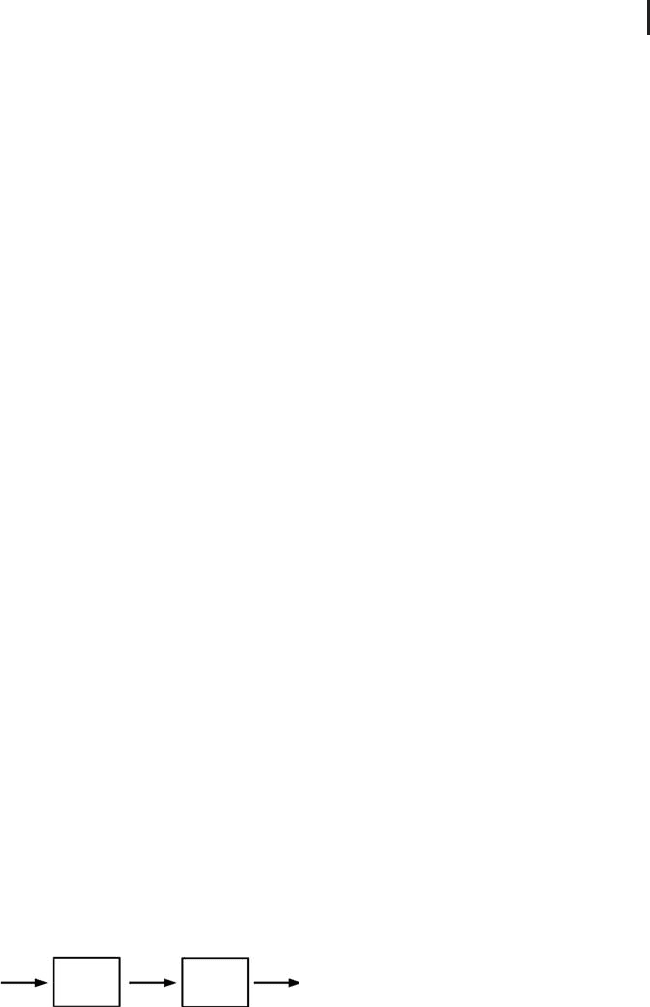
Typically, compartment models are visualized similar to Figure 3.23, that is, the

compartments are represented, for example, as rectangles, and arrows are used to

D(t)

G(t) B(t)

Fig. 3.23 Drug model as a two-compartment model.

226 3 Mechanistic Models I: ODEs

indicate the mutual exchange of mass, energy etc. between the compartments as

well as the mass and energy ﬂows between the compartments and the outside

world.

3.10.4

Plant Growth

A great number of mathematical models of plant growth has been developed, both

from the scientiﬁc perspective (for example: ‘‘how do plants grow?’’) and from

the engineering perspective (for example: ‘‘how can crop yield be maximized?’’),

see e.g. the books of Richter/S

ondgerath [41] and Overman/Scholtz [131], which

emphasize the scientiﬁc and engineering perspectives, respectively. In its simplest

form (which applies to plants and to other growing organisms in general), plant

growthmodelscanbewrittenintheform[41]



(t) = r · B(t) ·(B(t)) (3.309)

where B(t) denotes the overall biomass of the plant at time t (e.g. in kg ha

−1

), r

(e.g. in day

−1

) is the growth rate of the plant and (x) is some (dimensionless)

nonlinear real function. As usual, an initial condition is needed before this equation

can be solved, that is, we need to specify the value of the biomass at some time,

for example, in the form B(0) = B

. Depending on the choice of the function (B),

several plant growth models can be derived from Equation 3.309. For example ,

setting (B) = 1 generates the exponential growth model:



(t) = r · B(t) (3.310)

while (B) = 1 − B/K (for K ∈ R)givesthelogistic growth model:



(t) = r · B(t) ·



1 −

B(t)



(3.311)

Here, K (kg ha

−1

) can be interpreted as the (genetically ﬁxed) maximum possible

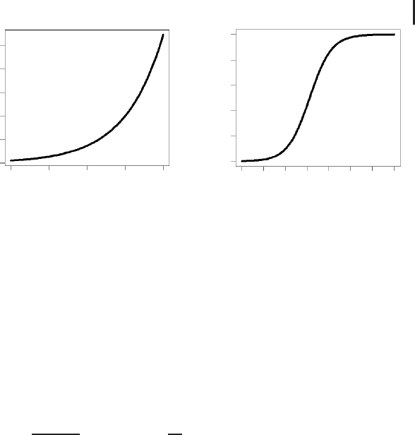
biomass of the plant. Figure 3.24 shows the typical patterns of the exponential and

logistic growth models. As can be seen, the exponential plant growth model yields

an exponential increase of the biomass, which holds true at the early stages of plant

growth. As the plant approaches its maximum possible biomass, the growth curve

will asymptotically slow down, which can be expressed using the logistic growth

model similar to Figure 3.24b.

Figure 3.24a,b has been produced using the codes

Plant1.r and Plant2.r

in the book software (see Appendix A), which were obtained by an appropriate

editing of

ODEEx1.r, and which are based on a numerical solution of the ODEs

Equations 3.310 and 3.311 (see Section 3.8.3). Of course, closed form solutions of

Equations 3.310 and 3.311 can also be easily obtained using the methods described

3.10 More Examples 227

100

B (kg ha

−1

)

200

300

400

500

B (kg ha

−1

)

10 20 30 40

t (days)

50 600 5 10 15

t (days)

(

)(

)

20 70

Fig. 3.24 Solutions (a) of the exponential plant growth

model, Equation 3.310 and (b) of the logistic plant growth

model, Equation 3.311 using: B(0) = 1, r = 0.2, K = 500

(plots generated using

Plant1.r and Plant2.r).

in Section 3.7. Assuming B(0) = B

as the initial condition, the closed form solution

of Equation 3.310 is

B(t) = B

(3.312)

and the closed form solution of Equation 3.311 is

B(t) =

1 +e

β−rt

where β = ln



− 1



(3.313)

A great number of plant growth models are obtained by appropriate modiﬁcations

of this approach, depending on the data that are analyzed and depending on the

question that one is asking. For example, multiorgan plant growth models can be

formulated basically by adding a growth model of the above kind for each of the

plant organs such as roots, stems, leaves and fruits, and by balancing the mass

ﬂows between these ‘‘compartments’’ following the idea of the compartmental

approach described in Section 3.10.3 above [41, 132, 133]. The above equations

can also be supplemented, for example, by equations describing the kinetics of

enzymes that are involved in photosynthesis if the focus of the investigation is on

air pollutants that affect these enzymes during plant growth [134, 135].

Different plant growth models may apply to one and the same plant depending on

the growth conditions. While the logistic growth model works well for the asparagus

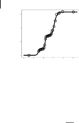
biomass data in [136], it was inapplicable to the staircase-like asparagus biomass

data shown in Figure 3.25. As discussed in [137], the staircase-like structure of the

data in the ﬁgure reﬂects the fact that several groups of asparagus spears had been

growing successively, that is, ﬁrst group 1 began to grow and stopped growing after

some time, then group 2 began to grow and stopped growing after some time and

so on. The data in Figure 3.25 look like several logistic growth functions stacked

on top of each other, and they can indeed be described by a system of ODEs that

228 3 Mechanistic Models I: ODEs

500

1000

1500

50 100 150

days

B (cm)

200 250

Fig. 3.25 Asparagus spear biomass data as-

paragus.csv compared with model Equations

3.314 and 3.315, where r

= 0.23, r

= 0.42,

= 0.15, K

= 230, K

= 480, K

= 870,

= 50, t

= 93, t

= 110, B

(0) = B

(0) =

(0) = 1. Data from [137] (note: biomass in

‘‘centimeter’’ based on a constant assumed

spear diameter and density). Plot generated

using

Plant3.r.

involves three logistic growth equations (one for three groups of spears in the above

sense) as follows:



(t) = r

· H(t − t

) ·



1 −

(t)



· B

(t)fori = 1, 2, 3 (3.314)

B(t) =



i=1

(t) (3.315)

where H(x) is the Heaviside step function that was introduced in Section 3.10.3.

Basically, the Heaviside function is used here to successively ‘‘switch on’’ the

growth functions for the three groups of asparagus spears. Figure 3.25 shows

an almost perfect coincidence of this model with the data. The ﬁgure has been

plotted using the code

Plant3.r in the book software, which is based on the

numerical solution of Equation 3.314 using

ODEEx1.r again (as before, the closed

form solution Equation 3.313 could also have been used to get the same result).

Note that the parameters shown in Figure 3.25 have been obtained from a (quick)

manual tuning of the parameters, although the (slightly more tedious) automated

procedure described in Section 3.9 could also have been used.

229

Mechanistic Models II: PDEs

4.1

Introduction

4.1.1

Limitations of ODE Models

Ordinary differential equation (ODE) models are restricted in the sense that they

involve derivatives with respect to one variable only, which means that they describe

the dynamical behavior of the quantity of interest with respect to this one variable

only. In the wine fermentation model, for example, the quantities of interest have

been the sugar, ethanol, nitrogen, and yeast cell biomass concentrations, and

all these quantities were considered as a function of time only (Section 3.10.2).

Looking at the examples in Section 3, you will note that time was the independent

variable in most examples, although, of course, any kind of variable can be used

in principal (e.g. a space coordinate was used as the independent variable in the

metal rod example, see Section 3.5.5)

Now, obviously, we live in a world where everything depends on many variables

simultaneously. Using ODE models, therefore, usually means we are referring to

special situations where it can be assumed that the independent variable used in

the ODE model is the most important factor affecting our quantity of interest, while

the inﬂuence of other factors with a possible impact on our quantity of interest

can be assumed to be negligible. In the wine fermentation model, for example, it

is obvious that quantities such as the yeast biomass concentration will depend not

only on time but also on the space coordinates x, y,andz. Assuming the yeast

biomass concentration would not depend on the spatial coordinates would require

that quantity to be exactly the same at every particular spatial coordinate within the

fermenter. You do not need to be a wine fermentation specialist to understand that

this is an unrealistic assumption, and that it may of course happen that you have

variable yeast biomass concentrations in the fermenter; for example, gravitation

may increase the yeast biomass at the bottom of the fermenter as discussed in [124].

The fact that the wine fermentation model – as well as the other ODE models

discussed in Section 3 – can be applied successfully in some situations, thus,

does not ‘‘prove’’ the spatial homogeneity of the state variables, or the absence

230 4 Mechanistic Models II: PDEs

of any other variables affecting the state variables. It just means that spatial

dishomogeneities, if they exist, and any other variables have a negligible effect

on your state variables in those particular situations where you apply the model

successfully. And you must always keep in mind that you are making a strong

assumption when you are neglecting all those other possible inﬂuences on your state

variables. This is particularly important when you observe deviations between your

model and data. In the wine fermentation model, substantial deviations from data

might indicate that you are, for example, in a situation where the dishomogeneity

of the yeast biomass concentration is so high that it can no longer be neglected.

Then a possible solution would be to use partial differential equations (PDEs),

which describe the dynamics of the yeast biomass concentration in time and space.

Note 4.1.1 (Limitations of ODE models) Deviations between an ODE model

and data may indicate that its state variables depend on more than one variable

(e.g. on time and space variables). Then, it may be appropriate to use PDE models

instead.

4.1.2

Overview: Strange Animals, Sounds, and Smells

In contrast to ODEs, PDE models involve derivatives with respect to at least two

independent variables, and hence they can be used to describe the dynamics of

your quantities of interest with respect to several variables at the same time. A great

number of the classical laws of nature can be formulated as PDEs, such as the

laws of planetary motion, thermodynamics, electrodynamics, ﬂuid ﬂow, elasticity,

and so on. As a whole, PDEs are a really big topic. In particular, their structure

is much more variable compared to ODEs since they involve several variables and

derivatives. There are many different subtypes of PDEs, which need speciﬁcally

tailored numerical procedures for their solution. Many volumes could be ﬁlled with

a thorough discussion of all those subtypes and their appropriate treatment, and

it is hence obvious that we need to conﬁne ourselves here to a ﬁrst introduction

into the topic, with the aim of introducing the reader to some of the main ideas

and procedures that are applied when people formulate and solve PDE models. If

you imagine the PDE topic as a dense and big jungle, then the intention of this

chapter can be described as cutting a small machete path, which you can follow to

get ﬁrst sensual impressions of those strange animals, sounds, and smells within

the jungle – so do not mistake yourself for a PDE expert after reading the following

pages. To know more about PDEs, readers are referred to an abundant literature

on the topic, for example, books such as [101, 138–142].

As a guide and compass for our machete path we will take the heat equation

that was already discussed in Section 3.5.5. This equation will serve as our main

example in the following introduction into PDEs and their numerical procedures.

The heat equation provides a way to compute temperature distributions, and since

so many processes in science and engineering are affected by temperature, it is

4.1 Introduction 231

important in all ﬁelds of science and engineering. This is why the two heat equation

problems posed in Section 4.1.3 really are ‘‘problems you should be able to solve’’.

Sections 4.2 and 4.3 provide some theoretical background on the heat equation

and on PDEs, in general. Sections 4.4–4.7 are devoted to the solution of PDEs

in closed form or based on numerical procedures, respectively. In Sections 4.8

and 4.9, software is discussed that solves PDEs based on the ﬁnite-element

method, which is one of the most important numerical procedures that can be

used to solve PDEs. Section 4.9 provides a sample session using the Salome-Meca

software, an open-source ﬁnite-element software with a general workﬂow similar

to commercial ﬁnite-element software (Appendix A). Then, Section 4.10 introduces

you to some of the most important PDE models ‘‘beyond the heat equation’’.

This includes, for example, computational ﬂuid dynamics (CFD) and structural

mechanics models and appropriate open-source software to solve these models

in 3D. Finally, Section 4.11 ends the chapter with some examples of mechanistic

modeling approaches beyond differential equations.

4.1.3

Two Problems You Should Be Able to Solve

We begin with the formulation of two problems that are solved below using PDEs,

and that will be used to motivate and illustrate the material in subsequent sections.

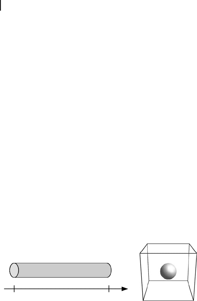
These problems are concerned with the computation of temperature distributions

in the geometries shown in Figure 4.1:

Problem 1:

Consider the cylinder in Figure 4.1a. Assuming

•

a perfect insulation of the cylinder surface in 0 < x < 1,

•

constant temperatures in the y and z directions at time t = 0,

that is, no temperature variations across transverse sections,

•

a known initial temperature distribution T

(x)attimet = 0,

•

and constant temperatures T

and T

at the left and right ends of

the cylinder for all times t > 0,

what is the temperature T(x, t)forx ∈ (0, 1) and t ∈ (0, T]?

Problem 2:

Referring to the conﬁguration in Figure 4.1b and assuming

•

a constant temperature T

at the top surface of the cube (z = 1),

•

a constant temperature T

atthespheresurface,

•

and a perfect insulation of all other surfaces of the cube,

what is the stationary temperature distribution T(x, y, z) within the cube (i.e. in

the domain [0, 1]

\ S if S is the sphere)?

232 4 Mechanistic Models II: PDEs

Note the practical relevance that problems of this kind have in both science and

engineering. As was mentioned above, PDEs are a very broad topic and involve a great

deal of really sophisticated mathematics. Taking one of the more mathematical

oriented books on PDEs, and then gazing at endless formulas, many of us will be

tempted to ask: ‘‘How can this be useful for me?’’ The above two problems give

the answer: PDEs are useful for everybody in science and engineering since they

provide the only way to solve absolutely fundamental and elementary problems

such as the computation of temperature distributions. No one can seriously doubt

the fundamental importance of temperature in science and engineering – just

remember, for example, the role of temperature in the wine fermentation model

discussed in Section 3.10.2. If you do not know how to solve this kind of problems,

then you lack to know one of the really fundamental methods in science and

engineering. Without too much exaggeration, one can say, it is a bit like not being

able to compute the surface area of a circle. Fortunately, you will be able to learn

about some PDE basics in this chapter from a very practical and software-oriented

point of view.

To make Problem 1 a little bit more concrete, you may imagine a situation

like this: the cylinder in Figure 4.1a is a metallic cylinder with a constant initial

temperature of 100

◦

C. At time t = 0, you keep the ends of the cylinder in ice water

◦

C) and maintain this situation unchanged for all times t > 0. Then, you know

that the temperature of the cylinder will be approximately 0

◦

C after ‘‘some time’’.

The problem is to make this precise, and to be able to predict temperatures at any

particular time t > 0 and at any particular location x ∈ (0, 1) within the cylinder.

Exactly this problem is solved in Section 4.6.

Regarding Problem 2, remember from the discussion of the metallic rod problem

in Section 3.5.5 the meaning of stationarity: the stationary temperature distribution

is what you obtain for t →∞if you do not change the environment. Referring

to Figure 4.1b, ‘‘unchanged environment’’ means that the temperatures imposed

at the top of the cube and at the sphere surface remain unchanged for all times

t > 0, the other sides of the cube remain perfectly insulated, and so on. Stationarity

(b)(a)

Fig. 4.1 (a) Cylinder used in Problem 1. (b) Cube

[0, 1]

, containing a cylinder with radius 0.1 centered at

(0.5, 0.5, 0.5), as used in Problem 2.

4.2 The Heat Equation 233

can also be explained referring to the above discussion of Problem 1,whereitwas

said that the temperature of the cylinder will be 0

◦

C after ‘‘some time’’, which can

be phrased as follows: given the conditions in the above discussion of Problem 1,

T(x) = 0

◦

C is the stationary solution, which is approached for t →∞(this will be

formally shown in Section 4.4).

Again, let us spend a few thoughts on what the situation in Problem 2 could

mean in a practical situation. As was said above, temperatures are of great

importance in all kinds of applications in science and engineering. Many of the

devices used in science and engineering contain certain parts specially designed

to control the temperature. The question then is whether the design of these

temperature-controlling parts is good enough in the sense that the resulting

temperature distribution in the device satisﬁes your needs. In Problem 2above,

the small sphere inside the cube can be viewed as a temperature-controlling part.

Once we are able to solve Problem 2, we can, for example, compare the resulting

temperature distribution with the distributions obtained if we use a small cube,

tetrahedron, and so on, instead of the sphere, and then try to optimize the design

of the temperature-controlling part in this way.

This procedure has been used, for example, in [143, 144] to optimize cultivation

measures affecting the temperature distribution in asparagus dams.Inthewine

fermentation example discussed above, temperature is one of the variables that is

used to control the process (Section 3.10.2). To be able to adjust temperatures

during fermentation, various cooling devices are used inside fermenters, and the

question then is where these cooling devices should be placed and how they should

be controlled such that the temperature distribution inside the fermenter meets

the requirements. In this example, the computation of temperature distributions

is further complicated by the presence of convectional ﬂows, which transport heat

through the fermenter. To compute temperature distributions in a situation like

this, we would have to solve a coupled problem, which would also involve the

computation of the ﬂuid ﬂow pattern in the fermenter. This underlines again that

Problem 2 can be seen as a ﬁrst approximation to a class of problems of great

practical importance.

4.2

The Heat Equation

To solve the problems posed in Section 4.1.3, we need an equation that describes

the dynamics of temperature as a function of space and time: the heat equation.

The heat equation is used here in the following form:

∂T

∂t

Cρ



∂

∂x

∂

∂y

∂

∂z



(4.1)

where K (WK

−1

) is the thermal conductivity, C (J kg

−1

) is the speciﬁc heat

capacity, and ρ (kg m

−3

) is the density.

234 4 Mechanistic Models II: PDEs

Using the so-called Laplace operator

 =

∂

∂x

∂

∂y

∂

∂z

(4.2)

the heat equation is also frequently written as

∂T

∂t

Cρ

T (4.3)

We could end our discussion of the heat equation here (before it actually begins)

and work with this equation as it is. That is, we could immediately turn to the

mathematical question of how this equation can be solved, and how it can be

applied to the problems in Section 4.1.3. Indeed, the reader could skip the rest of

this section and continue with Section 4.3 if he or she is interested in the technical

aspects of solving this kind of problems. It is, nevertheless, recommended to read

the rest of this section, not only because it is always good to have an idea about the

background of the equations that one is using. The following discussion introduces

you into an important way how this and many other PDEs can be derived from

balance considerations, and beyond this you will understand why most PDEs in

the applications are of second order.

4.2.1

Fourier’s Law

The speciﬁc heat capacity C in the above equations is a measure of the amount

of heat energy required to increase the temperature of 1 kg of the material under

consideration by 1

◦

C. Values of C can be found in the literature, as well as values

for the thermal conductivity K, which is the proportionality constant in an empirical

relation called Fouriers’s law:

⎛

⎜

⎝

⎞

⎟

⎠

=−K ·

⎛

⎜

⎝

∂T

∂x

∂T

∂y

∂T

∂z

⎞

⎟

⎠

(4.4)

Using q = (q

, q

)

and the nabla operator

∇=

⎛

⎜

⎝

∂

∂x

∂

∂y

∂

∂z

⎞

⎟

⎠

(4.5)