Versteeg H., Malalasekra W. An Introduction to Computational Fluid Dynamics: The Finite Volume Method

Подождите немного. Документ загружается.

5.11 SUMMARY 177

• The boundary conditions enter the discretised equations via source

terms. Their treatment is speciﬁc to each discretisation scheme.

• Discretisation schemes that possess conservativeness, boundedness and

transportiveness give physically realistic results and stable iterative

solutions:

– The central differencing method is not suitable for general-purpose

convection–diffusion problems because it lacks transportiveness and

gives unrealistic solutions at large values of the cell Peclet number.

– Upwind, hybrid and power-law differencing all possess

conservativeness, boundedness and transportiveness and are highly

stable, but suffer from false diffusion in multi-dimensional ﬂows if

the velocity vector is not parallel to one of the co-ordinate

directions.

• The discretised equations of the standard QUICK method of Leonard

(1979) have the following form for a general internal node point:

= a

+ a

(5.87)

where

= a

+ a

+ (F

− F

)

The neighbour coefﬁcients of the standard QUICK scheme are

Standard QUICK

+ (1 −

−

− (1 −

(1 −

with

= 1 for F

> 0 and

= 1 for F

> 0

= 0 for F

< 0 and

= 0 for F

< 0

• Higher-order schemes, such as QUICK, can minimise false diffusion

errors but are less computationally stable. This manifests itself as

small over- and undershoots in the solution of some problems

including those with large gradients of

, which can potentially lead to

non-physical behaviour, e.g. negative turbulence properties k and

in extreme cases. Nevertheless, if used with care and judgement the

QUICK scheme can give very accurate solutions of

convection–diffusion problems.

ANIN_C05.qxd 29/12/2006 04:36PM Page 177

178 CHAPTER 5 FINITE VOLUME METHOD FOR C---D PROBLEMS

• The discretised equations of the TVD schemes have the following form

for a general internal node point:

= a

+ a

+ S

(5.88)

where

= a

+ a

+ (F

− F

)

The neighbour coefﬁcients and deferred correction source term of TVD

schemes are as follows:

TVD neighbour coefﬁcients

= D

+ max(F

, 0)

= D

+ max(−F

, 0)

TVD deferred correction source term

–

[(1 −

)

−

) −

)](

−

)

–

[

) − (1 −

)

−

)](

−

)

with

= 1 for F

> 0 and

= 1 for F

> 0

= 0 for F

< 0 and

= 0 for F

< 0

• The most frequently used limiter functions are

Name Limiter function

ψψ

(r)

Van Leer

Van Albada

Min-Mod

(r) =

min(r, 1) if r > 0

0 if r ≤ 0

Roe’s SUPERBEE max[0, min(2r, 1), min(r, 2)]

Sweby max[0, min(

r, 1), min(r,

)]

QUICK max[0, min(2r, (3 + r)/4, 2)]

UMIST max[0, min(2r, (1+ 3r)/4, (3 + r)/4, 2)]

• The performance of the limiter functions has been found to be fairly

similar: all TVD discretisations based on the above limiter functions

give second-order accurate solutions that are free from non-physical

wiggles, so all are suitable for general-purpose CFD computations.

r + r

1 + r

r +|r|

1 + r

ANIN_C05.qxd 29/12/2006 04:36PM Page 178

The convection of a scalar variable

depends on the magnitude and direc-

tion of the local velocity ﬁeld. To develop our methods in the previous chap-

ter we assumed that the velocity ﬁeld was somehow known. In general the

velocity ﬁeld is, however, not known and emerges as part of the overall solu-

tion process along with all other ﬂow variables. In this chapter we look at the

most popular strategies for computing the entire ﬂow ﬁeld.

Transport equations for each velocity component – momentum equations

– can be derived from the general transport equation (2.39) by replacing the

variable

by u, v and w respectively. Every velocity component appears in

each momentum equation, and the velocity ﬁeld must also satisfy the con-

tinuity equation. This can be clearly shown by considering the equations

governing a two-dimensional laminar steady ﬂow:

x-momentum equation

(

uu) + (

vu) =

−+S

(6.1)

y-momentum equation

(

uv) + (

vv) =

−+S

(6.2)

continuity equation

(

u) + (

v) = 0 (6.3)

The pressure gradient term, which forms the main momentum source term

in most ﬂows of engineering importance, has been written separately to

facilitate the discussion that follows.

The solution of equation set (6.1)–(6.3) presents us with two new problems:

• The convective terms of the momentum equations contain non-linear

quantities: for example, the ﬁrst term of equation (6.1) is the x-

derivative of

• All three equations are intricately coupled because every velocity

component appears in each momentum equation and in the continuity

equation. The most complex issue to resolve is the role played by the

∂

Chapter six Solution algorithms for pressure---

velocity coupling in steady flows

Introduction6.1

ANIN_C06.qxd 29/12/2006 09:59 AM Page 179

pressure. It appears in both momentum equations, but there is evidently

no (transport or other) equation for the pressure.

If the pressure gradient is known, the process of obtaining discretised equa-

tions for velocities from the momentum equations is exactly the same as that

for any other scalar, and the schemes explained in Chapter 5 are applicable.

In general-purpose ﬂow computations we also wish to calculate the pressure

ﬁeld as part of the solution, so its gradient is not normally known beforehand.

If the ﬂow is compressible the continuity equation may be used as the trans-

port equation for density and, in addition to (6.1)–(6.3), the energy equation

is the transport equation for temperature. The pressure may then be obtained

from density and temperature by using the equation of state p = p(

, T ).

However, if the ﬂow is incompressible the density is constant and hence by

deﬁnition not linked to the pressure. In this case coupling between pressure

and velocity introduces a constraint in the solution of the ﬂow ﬁeld: if the

correct pressure ﬁeld is applied in the momentum equations the resulting

velocity ﬁeld should satisfy continuity.

Both the problems associated with the non-linearities in the equation set

and the pressure–velocity linkage can be resolved by adopting an iterative

solution strategy such as the SIMPLE algorithm of Patankar and Spalding

(1972). In this algorithm the convective ﬂuxes per unit mass F through cell

faces are evaluated from so-called guessed velocity components. Further-

more, a guessed pressure ﬁeld is used to solve the momentum equations, and

a pressure correction equation, deduced from the continuity equation, is

solved to obtain a pressure correction ﬁeld, which is in turn used to update

the velocity and pressure ﬁelds. To start the iteration process we use initial

guesses for the velocity and pressure ﬁelds. As the algorithm proceeds our

aim must be progressively to improve these guessed ﬁelds. The process

is iterated until convergence of the velocity and pressure ﬁelds. The main

features of the SIMPLE algorithm and its more recent enhancements will be

discussed in this chapter.

The solution procedure for the transport of a general property

developed

in Chapter 5 will, of course, be enlisted to solve the momentum equations.

Matters are, however, not completely straightforward since there are prob-

lems associated with the pressure source terms of the momentum equations

that need special treatment.

The ﬁnite volume method starts, as always, with the discretisation of the

ﬂow domain and of the relevant transport equations (6.1)–(6.3). First we

need to decide where to store the velocities. It seems logical to deﬁne these

at the same locations as the scalar variables such as pressure, temperature

etc. However, if velocities and pressures are both deﬁned at the nodes of an

ordinary control volume a highly non-uniform pressure ﬁeld can act like a

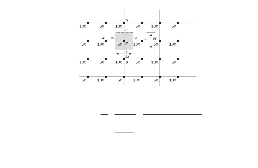
uniform ﬁeld in the discretised momentum equations. This can be demon-

strated with the simple two-dimensional situation shown in Figure 6.1,

where a uniform grid is used for simplicity. Let us assume that we have

somehow obtained a highly irregular ‘checker-board’ pressure ﬁeld with

values as shown in Figure 6.1.

If pressures at e and w are obtained by linear interpolation the pressure

gradient term

∂

x in the u-momentum equation is given by

180 CHAPTER 6 ALGORITHMS FOR PRESSURE---VELOCITY COUPLING

The staggered

grid

6.2

ANIN_C06.qxd 29/12/2006 09:59 AM Page 180

6.2 THE STAGGERED GRID 181

−

= (6.4)

Similarly, the pressure gradient

∂

y for the v-momentum equation is

evaluated as

= (6.5)

The pressure at the central node (P) does not appear in (6.4) and (6.5).

Substituting the appropriate values from the ‘checker-board’ pressure ﬁeld

in Figure 6.1 into (6.4)–(6.5) we ﬁnd that all the discretised gradients are

zero at all the nodal points even though the pressure ﬁeld exhibits spatial

oscillations in both directions. As a result, this pressure ﬁeld would give the

same (zero) momentum source in the discretised equations as a uniform

pressure ﬁeld. This behaviour is obviously non-physical.

It is clear that, if the velocities are deﬁned at the scalar grid nodes, the

inﬂuence of pressure is not properly represented in the discretised momentum

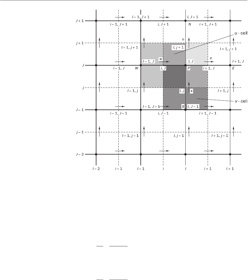
equations. A remedy for this problem is to use a staggered grid for velocity

components (Harlow and Welch, 1965). The idea is to evaluate scalar vari-

ables, such as pressure, density, temperature etc., at ordinary nodal points

but to calculate velocity components on staggered grids centred around the

cell faces. The arrangement for a two-dimensional ﬂow calculation is shown

in Figure 6.2.

The scalar variables, including pressure, are stored at the nodes marked

(

•

). The velocities are deﬁned at the (scalar) cell faces in between the nodes

and are indicated by arrows. Horizontal (→) arrows indicate the locations for

u-velocities and vertical (↑) ones denote those for v-velocity. In addition to

the E, W, N, S notation Figure 6.2 also introduces a new system of notation

based on a numbering of grid lines and cell faces. It will be explained and

used later on in this chapter.

For the moment we continue to use the original E, W, N, S notation; the

u-velocities are stored at scalar cell faces e and w and the v-velocities at

faces n and s. In a three-dimensional ﬂow the w-component is evaluated

at cell faces t and b. We observe that the control volumes for u and v are

− p

∂

− p

∂

+ p

Figure 6.1 A ‘checker-board’

pressure ﬁeld

ANIN_C06.qxd 29/12/2006 09:59 AM Page 181

different from the scalar control volumes and from each other. The scalar

control volumes are sometimes referred to as the pressure control volumes

because, as we will see later, the discretised continuity equation is turned

into a pressure correction equation, which is evaluated on scalar control

volumes.

In the staggered grid arrangement, the pressure nodes coincide with

the cell faces of the u-control volume. The pressure gradient term

∂

x is

given by

= (6.6)

where

is the width of the u-control volume. Similarly

∂

y for the v-

control volume shown is given by

= (6.7)

where

is the width of the v-control volume.

If we consider the ‘checker-board’ pressure ﬁeld again, substitution of the

appropriate nodal pressure values into equations (6.6) and (6.7) now yields

very signiﬁcant non-zero pressure gradient terms. The staggering of the

velocity avoids the unrealistic behaviour of the discretised momentum equa-

tion for spatially oscillating pressures like the ‘checker-board’ ﬁeld. A further

advantage of the staggered grid arrangement is that it generates velocities at

− p

∂

− p

∂

182 CHAPTER 6 ALGORITHMS FOR PRESSURE---VELOCITY COUPLING

Figure 6.2

ANIN_C06.qxd 29/12/2006 09:59 AM Page 182

6.3 THE MOMENTUM EQUATIONS 183

exactly the locations where they are required for the scalar transport –

convection–diffusion – computations. Hence, no interpolation is needed to

calculate velocities at the scalar cell faces.

As mentioned earlier, if the pressure ﬁeld is known, the discretisation of

velocity equations and the subsequent solution procedure is the same as that

of a scalar equation. Since the velocity grid is staggered the new notation

based on grid line and cell face numbering will be used. In Figure 6.2

the unbroken grid lines are numbered by means of capital letters. In the

x-direction the numbering is ..., I − 1, I, I + 1, . . . etc. and in the y-

direction ..., J − 1, J, J + 1, . . . etc. The dashed lines that construct the cell

faces are denoted by lower case letters ..., i − 1, i, i + 1,...and..., j − 1,

j, j + 1, . . . in the x- and y-directions respectively.

A subscript system based on this numbering allows us to deﬁne the loca-

tions of grid nodes and cell faces with precision. Scalar nodes, located at the

intersection of two grid lines, are identiﬁed by two capital letters: e.g. point

P in Figure 6.2 is denoted by (I, J ). The u-velocities are stored at the e- and

w-cell faces of a scalar control volume. These are located at the intersection

of a line deﬁning a cell boundary and a grid line and are, therefore, deﬁned

by a combination of a lower case letter and a capital, e.g. the w-face of the cell

around point P is identiﬁed by (i, J). For the same reasons the storage loca-

tions for the v-velocities are combinations of a capital and a lower case letter:

e.g. the s-face is given by (I, j).

We may use forward or backward staggered velocity grids. The uniform

grids in Figure 6.2 are backward staggered since the i-location for the

u-velocity u

i, J

is at a distance of −

–

from the scalar node (I, J). Likewise,

the j-location for the v-velocity v

I, j

is −

–

from node (I, J ).

Expressed in the new co-ordinate system the discretised u-momentum

equation for the velocity at location (i, J ) is given by

i, J

=∑a

−∆V

+ D∆V

i, J

=∑a

+ (p

I−1, J

− p

I, J

i, J

+ b

i, J

(6.8)

where ∆V

is the volume of the u-cell, b

i, J

= D∆V

is the momentum source

term, A

i, J

is the (east or west) cell face area of the u-control volume. The

pressure gradient source term in (6.8) has been discretised by means of a

linear interpolation between the pressure nodes on the u-control volume

boundaries.

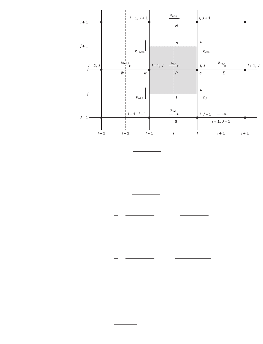
In the new numbering system the E, W, N and S neighbours involved in

the summation ∑a

are (i − 1, J), (i + 1, J), (i, J − 1) and (i, J + 1). Their

locations and the prevailing velocities are shown in more detail in Figure 6.3.

The values of coefﬁcients a

i, J

and a

may be calculated with any of the

differencing methods (upwind, hybrid, QUICK, TVD) suitable for con-

vection–diffusion problems. The coefﬁcients contain combinations of the

convective ﬂux per unit mass F and the diffusive conductance D at u-control

volume cell faces. Applying the new notation system we give the values of F

and D for each of the faces e, w, n and s of the u-control volume:

I, J

− p

I−1, J

The momentum

equations

6.3

ANIN_C06.qxd 29/12/2006 09:59 AM Page 183

= (

= u

i, J

+ u

i−1, J

(6.9a)

= (

= u

i+1, J

+ u

i, J

(6.9b)

= (

= v

I, j

+ v

I−1, j

(6.9c)

= (

= v

I, j+1

+ v

I−1, j+1

(6.9d)

= (6.9e)

= (6.9f )

I, J

i+1

− x

I−1, J

− x

i −1

I−1, J+1

I−1, J

I, J+1

I, J

I, j+1

+ F

I−1, j+1

I−1, J

I−1, J−1

I, J

I, J−1

I, j

+ F

I−1, j

I, J

I−1, J

I+1, J

I, J

i+1, J

+ F

i, J

I−1, J

I−2, J

I, J

I−1, J

i, J

+ F

i −1, J

184 CHAPTER 6 ALGORITHMS FOR PRESSURE---VELOCITY COUPLING

Figure 6.3 A u-control volume

and its neighbouring velocity

components

ANIN_C06.qxd 29/12/2006 09:59 AM Page 184

6.3 THE MOMENTUM EQUATIONS 185

= (6.9g)

= (6.9h)

The formulae (6.9) show that where scalar variables or velocity components

are not available at a u-control volume cell face, a suitable two- or four-point

average is formed over the nearest points where values are available. During

each iteration the u- and v-velocity components used to evaluate the above

expressions are those obtained as the outcome of the previous iteration (or

the initial guess in the ﬁrst iteration). It should be noted that these known

u- and v-values contribute to the coefﬁcients a in equation (6.8). These are

distinct from u

i, J

and u

in this equation, which denote the unknown scalars.

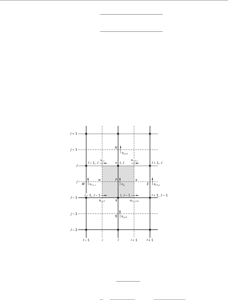
By analogy the v-momentum equation becomes

I, j

=∑a

+ (p

I, J−1

− p

I, J

I, j

+ b

I, j

(6.10)

The neighbours involved in the summation ∑a

and prevailing velocities

are as shown in Figure 6.4.

I−1, J+1

+Γ

I, J+1

+Γ

I−1, J

+Γ

I, J

4( y

J+1

− y

)

I−1, J

+Γ

I, J

+Γ

I−1, J−1

+Γ

I, J−1

4( y

− y

J−1

)

Figure 6.4 A v-control volume

and its neighbouring velocity

components

Coefﬁcients a

I, j

and a

again contain combinations of the convective ﬂux

per unit mass F and the diffusive conductance D at v-control volume cell

faces. Their values are obtained by the same averaging procedure adopted for

the u-control volume and are given below:

= (

= u

i, J

+ u

i, J −1

(6.11a)

I−1, J−1

I, J−1

I, J

I−1, J

i, J

+ F

i, J−1

ANIN_C06.qxd 29/12/2006 09:59 AM Page 185

186 CHAPTER 6 ALGORITHMS FOR PRESSURE---VELOCITY COUPLING

The SIMPLE

algorithm

6.4

= (

= u

i+1, J

+ u

i+1, J −1

(6.11b)

= (

= v

I, j−1

+ v

I, j

(6.11c)

= (

= v

I, j

+ v

I, j+1

(6.11d)

= (6.11e)

= (6.11f )

= (6.11g)

= (6.11h)

Again at each iteration level the values of F are computed using the u- and

v- velocity components resulting from the previous iteration.

Given a pressure ﬁeld p, discretised momentum equations of the form

(6.8) and (6.10) can be written for each u- and v-control volume and then

solved to obtain the velocity ﬁelds. If the pressure ﬁeld is correct the result-

ing velocity ﬁeld will satisfy continuity. As the pressure ﬁeld is unknown, we

need a method for calculating pressure.

The acronym SIMPLE stands for Semi-Implicit Method for Pressure-

Linked Equations. The algorithm was originally put forward by Patankar

and Spalding (1972) and is essentially a guess-and-correct procedure for the

calculation of pressure on the staggered grid arrangement introduced above.

The method is illustrated by considering the two-dimensional laminar steady

ﬂow equations in Cartesian co-ordinates.

To initiate the SIMPLE calculation process a pressure ﬁeld p* is guessed.

Discretised momentum equations (6.8) and (6.10) are solved using the

guessed pressure ﬁeld to yield velocity components u* and v* as follows:

i, J

u *

i, J

=∑a

+ (p *

I−1, J

− p *

I, J

i, J

+ b

i, J

(6.12)

I, J

j+1

− y

I, J−1

− y

j−1

I, J−1

+Γ

I+1, J−1

+Γ

I, J

+Γ

I+1, J

4(x

I+1

− x

)

I−1, J−1

+Γ

I, J−1

+Γ

I−1, J

+Γ

I, J

4(x

− x

I−1

)

I, J+1

I, J

I, J−1

I, j

+ F

I, j+1

I, J

I, J−1

I, J−2

I, j−1

+ F

I, j

I, J−1

I+1, J−1

I+1, J

I, J

i+1, J

+ F

i+1, J −1

ANIN_C06.qxd 29/12/2006 09:59 AM Page 186