Versteeg H., Malalasekra W. An Introduction to Computational Fluid Dynamics: The Finite Volume Method
Подождите немного. Документ загружается.

6.10 WORKED EXAMPLES OF THE SIMPLE ALGORITHM 197
To illustrate the workings of the SIMPLE algorithm we give two detailed
examples. To restrict the number of individual calculations we limit our-
selves to one-dimensional flows as we have done in Chapters 4 and 5. In the
first example we show how to update a velocity field in the case of a friction-
less, incompressible flow through a duct of constant cross-sectional area.
This problem has a trivial solution of constant velocity, but the example
shows how an initial guess with varying velocities along the length of the
duct is updated to satisfy mass conservation using the pressure correction
equation. The second example looks at the frictionless, incompressible flow
through a planar, converging nozzle. The nozzle shape cannot be accurately
represented in the Cartesian x–y coordinate system that we have used until
now. However, by making the assumption that the flow is unidirectional and
all flow variables are uniformly distributed throughout every cross-section
perpendicular to the flow direction, we can develop a set of one-dimensional
governing equations for the problem. These exhibit the same pressure–
velocity coupling issues as the two- and three-dimensional Navier–Stokes
equations. Iterative solution of the discretised momentum equation and the
pressure correction equation is needed to obtain the velocity and pressure
field. We check the accuracy of the computed solution for our second
example against the well-known Bernoulli equation.
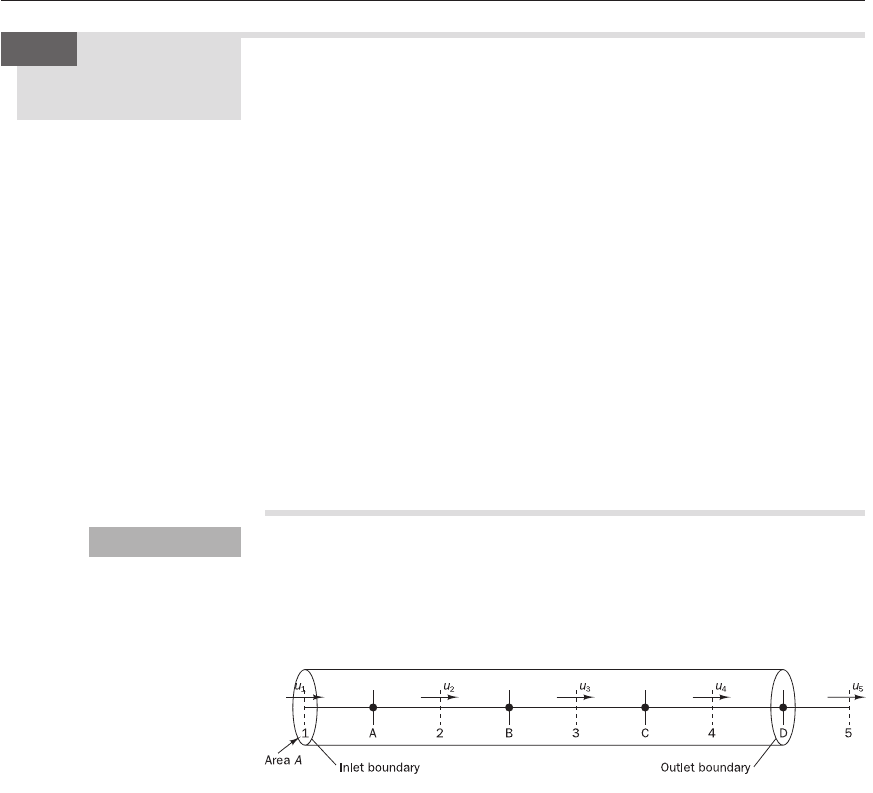
We consider the steady, one-dimensional flow of a constant-density fluid
through a duct with constant cross-sectional area. We use the staggered grid
shown in Figure 6.9, where the pressure p is evaluated at the main nodes
I = A, B, C and D, whilst the velocity u is calculated at the backward
staggered nodes i = 1, 2, 3 and 4.
Worked examples
of the SIMPLE
algorithm
6.10
Example 6.1
Figure 6.9
As a starting point we assume that we have used a guessed pressure field
p* in the discretised momentum equation to obtain a guessed velocity field
u*. In this example we demonstrate the guess-and-correct procedure that
forms the basis of the SIMPLE algorithm. Equation (6.32) is applied to
generate pressure corrections p′, which in turn yield velocity corrections u′
by means of
u′=d(p ′
I
− p ′
I+1
) (6.59)
and hence the corrected velocity field
u = u* + u′ (6.60)
Problem data
The problem data are as follows:
• Density
ρ
= 1.0 kg/m
3
is constant.
• Duct area A is constant.
ANIN_C06.qxd 29/12/2006 09:59 AM Page 197

• Multiplier d in equation (6.59) is assumed to be constant; we take d = 1.0.
• Boundary conditions: u
1
= 10 m/s and p
D
= 0 Pa.
• Initial guessed velocity field: say u
2
* = 8.0 m/s, u
3
* = 11.0 m/s and
u
4
* = 7.0 m/s.
Use the SIMPLE algorithm and these problem data to calculate pressure
corrections at nodes I = A to D and obtain the corrected velocity field at
nodes i = 2 to 4. In this very straightforward problem with constant area
and constant density it is easy to see that the velocity must be constant
everywhere by continuity. Hence, we will be able to compare our computed
solution against the exact solution u
2
= u
3
= u
4
= 10 m/s.
The pressure correction equation for this one-dimensional situation is
equation (6.32):
a
P
p ′
P
= a
W
p ′
W
+ a
E
p ′
E
+ b′
where a
W
= (
ρ
dA)
w
, a
E
= (
ρ
dA)
e
, a
P
= a
W
+ a
E
and b′=(
ρ
u*A)
w
− (
ρ
u*A)
e
Nodes B and C are internal nodes.
Node B
a
W
= (
ρ
dA)
w
= (
ρ
dA)
2
= 1.0 × 1.0 × A = 1.0A
a
E
= (
ρ
dA)
e
= (
ρ
dA)
3
= 1.0 × 1.0 × A = 1.0A
a
P
= a
W
+ a
E
= 1.0A + 1.0A = 2.0A
b′=(
ρ
u*A)
w
− (
ρ
u*A)
e
= (
ρ
u*A)
2
− (
ρ
u*A)
3
= (1.0 × 8. × A) − (1.0 × 11. × A) =−3.0A
The discretised pressure correction equation at node B is
(2.0A)p ′
B
= (1.0A)p ′
A
+ (1.0A)p ′
C
+ (−3.0A)
The area A cancels on the left and right hand sides, which yields
2p ′
B
= p ′
A
+ p ′
C
− 3
Node C
a
W
= (
ρ
dA)
w
= (
ρ
dA)
3
= 1.0 × 1.0 × A = 1.0A
a
E
= (
ρ
dA)
e
= (
ρ
dA)
4
= 1.0 × 1.0 × A = 1.0A
a
P
= a
W
+ a
E
= 1.0A + 1.0A = 2.0A
b′=(
ρ
u*A)
w
− (
ρ
u*A)
e
= (
ρ
u*A)
3
− (
ρ
u*A)
4
= (1.0 × 11. × A) − (1.0 × 7. × A) = 4.0A
The discretised pressure correction equation at node C is
(2.0A)p ′
C
= (1.0A)p ′
B
+ (1.0A)p ′
D
+ (4.0A)
2p ′
C
= p ′
B
+ p ′
D
+ 4
Nodes A and D are boundary nodes.
Node A
We cut the link to the west boundary side by setting the relevant coefficient
to zero and introduce the appropriate flux, in this case the mass flow rate into
the control volume through the boundary side, as a source term b′.
198 CHAPTER 6 ALGORITHMS FOR PRESSURE---VELOCITY COUPLING
Solution
ANIN_C06.qxd 29/12/2006 09:59 AM Page 198

6.10 WORKED EXAMPLES OF THE SIMPLE ALGORITHM 199
a
W
= 0.0
a
E
= (
ρ
dA)
e
= (
ρ
dA)
2
= 1.0 × 1.0 × A = 1.0A
a
P
= a
W
+ a
E
= 0.0 + 1.0A = 1.0A
b′=(
ρ
u*A)
w
− (
ρ
u*A)
e
+ (
ρ
uA)
boundary
=−(
ρ
u*A)
2
+ (
ρ
uA)
1
=
=−(1.0 × 8. × A) + (1.0 × 10. × A)
= 2.0A
Note that the given velocity at node 1 has been used in the calculation of the
additional source contribution to b′. Using the above we obtain the discre-
tised pressure correction equation at node A as
(1.0A)p′
A
= 0 + (1.0A)p′
B
+ (2.0A)
p′
A
= p′
B
+ 2.0
Node D
The boundary condition at node D is fixed pressure p
D
= 0. Since we know
the pressure we do not need a pressure correction: hence at node D we have
p′
D
= 0.
Thus we need to solve the following system of four equations for the four
pressure corrections:
p′
A
= p′
B
+ 2
2p′
B
= p′
A
+ p′
C
− 3
2p′
C
= p′
B
+ p′
D
+ 4
p′
D
= 0
We use p′
D
= 0 directly in the pressure correction equation for node C, which
becomes
2p′
C
= p′
B
+ 4
This leaves a system of three equations with three unknowns. In matrix form
the pressure correction equations are
G 1 −10JGp ′
A
JG2J
H−12−1KHp′
B
K = H−3K
I 0 −12LIp ′
C
LI4L
Solution of this set of equations gives
p ′
A
= 4.0, p ′
B
= 2.0 and p ′
C
= 3.0 (with p′
D
= 0 as before).
We obtain corrected velocities by combining (6.59) with (6.60):
u = u* + d(p′
I
− p′
I+1
)
Substitution of the problem data and the computed values for p′ yields
Velocity node 2: u
2
= u*
2
+ d(p′
A
− p′
B
) = 8.0 + 1.0 × [4.0 − 2.0] = 10.0 m/s
Velocity node 3: u
3
= u*
3
+ d(p′
B
− p′
C
) = 11.0 + 1.0 × [2.0 − 3.0] = 10.0 m/s
Velocity node 4: u
4
= u*
4
+ d(p′
C
− p′
D
) = 7.0 + 1.0 × [3.0 − 0.0] = 10.0 m/s
This shows how the guess-and-correct procedure gives the exact velocity
field in a single iteration for this very simple example. In more general flow
ANIN_C06.qxd 29/12/2006 09:59 AM Page 199
problems the pressure and velocity fields are coupled, so the pressure
correction equation must be solved along with the discretised momentum
equations. Furthermore, we note that the value of d in expression (6.59) for
the velocity corrections was assumed to be constant. Normally, the value of
d will vary from node to node and must be calculated with (6.23) and (6.28)
using control volume face areas and central coefficient (a
P
) values from the
discretised momentum equations. This process will be illustrated in the next
example.
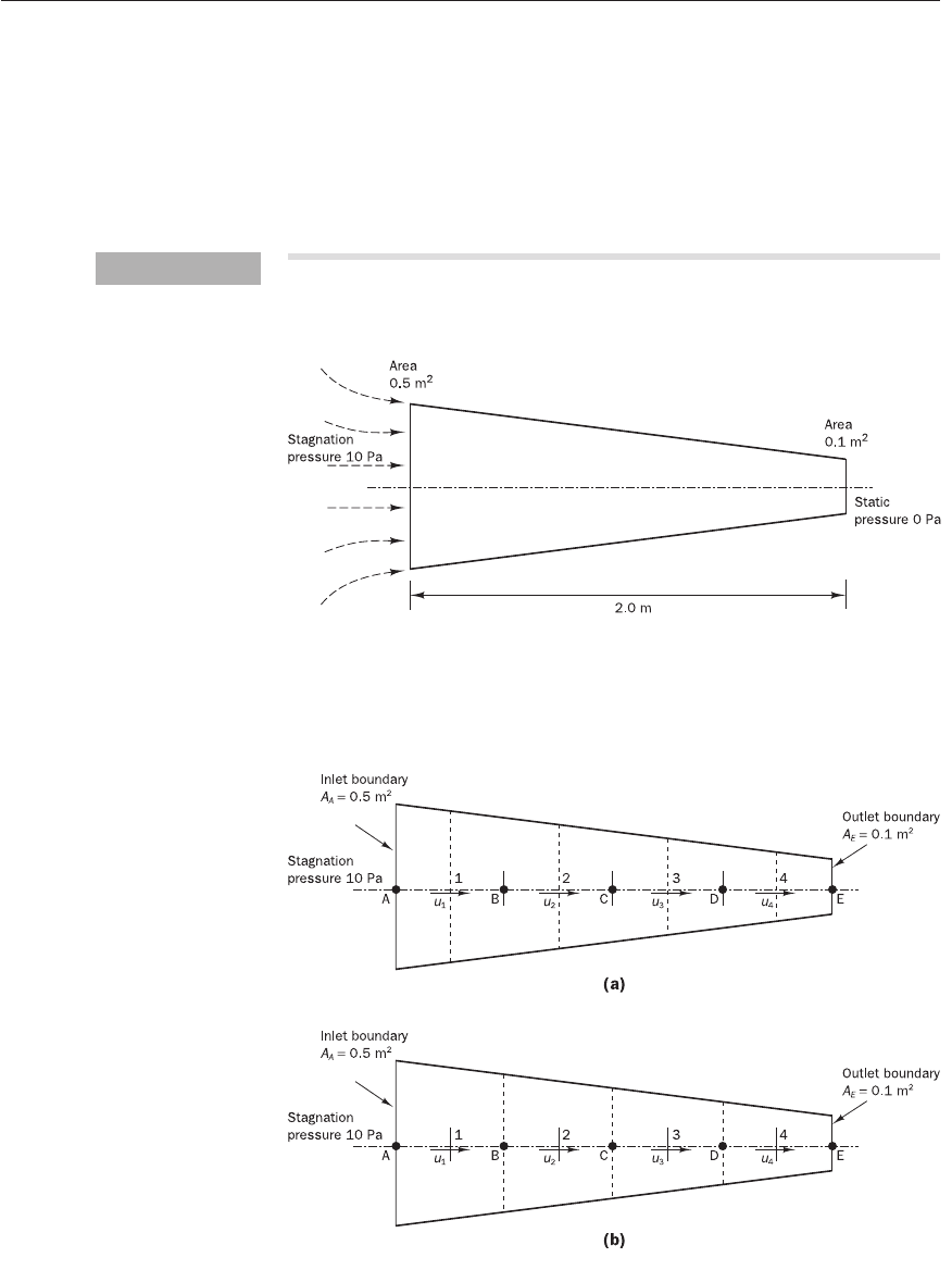
A planar two-dimensional nozzle is shown in Figure 6.10. The flow is steady
and frictionless and the density of the fluid is constant.
200 CHAPTER 6 ALGORITHMS FOR PRESSURE---VELOCITY COUPLING
Figure 6.10 Geometry of planar
2D nozzle
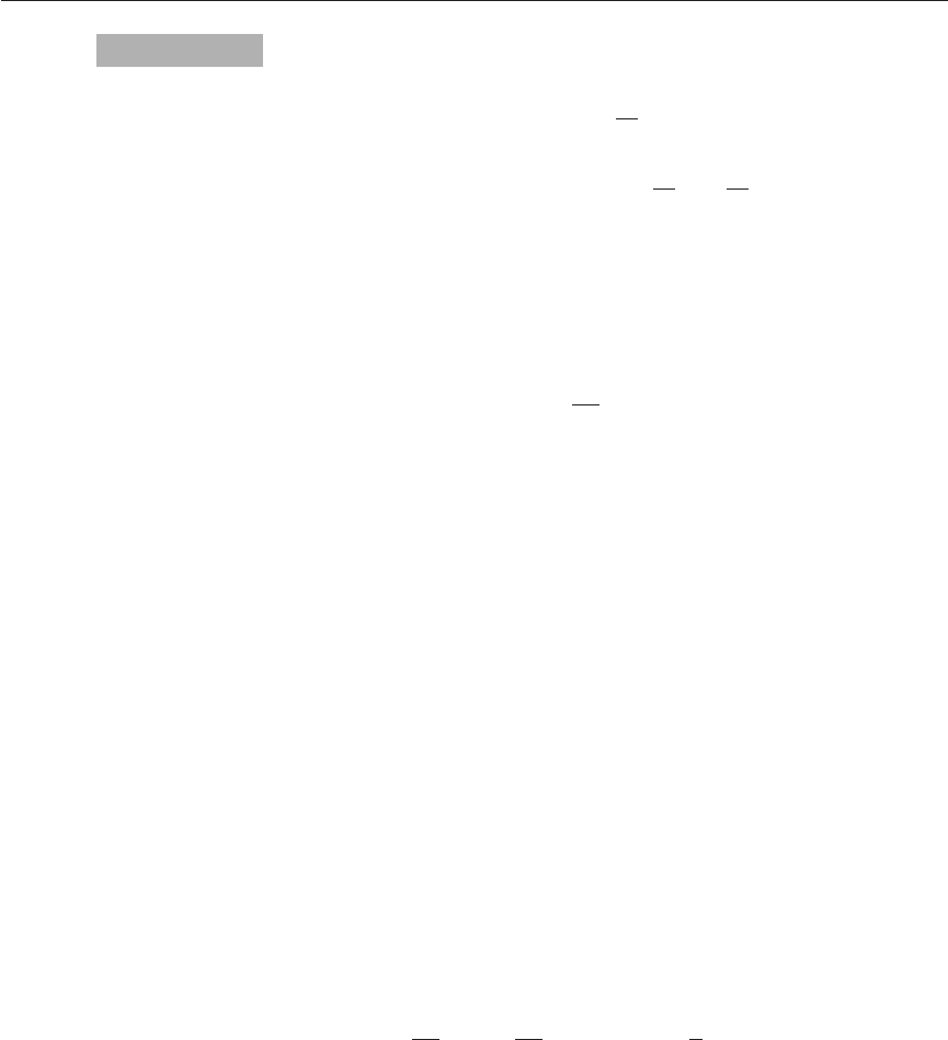
Figure 6.11 (a) The grid for
pressure control volumes; (b) the
grid for velocity control volumes
Example 6.2
Use the backward-staggered grid with five pressure nodes and four
velocity nodes shown in Figures 6.11a–b. The stagnation pressure is given at
the inlet and the static pressure is specified at the exit. Using the SIMPLE
ANIN_C06.qxd 29/12/2006 09:59 AM Page 200

6.10 WORKED EXAMPLES OF THE SIMPLE ALGORITHM 201
algorithm write down the discretised momentum and pressure correction
equations and solve for the unknown pressures at nodes I = B, C and D
and velocities at nodes i = 1, 2, 3 and 4. Check whether the computed velo-
city field satisfies continuity and evaluate the error in the computed pressure
and velocity fields by comparing with the exact solution.
Problem data
• The density of the fluid is 1.0 kg/m
3
.
• Grid spacing: nozzle length L = 2.00 m. The grid is uniform so
∆x = L/4 = 2.00/4 = 0.5 m.
• Cross-sectional area at the inlet A
A
= 0.5 m
2
and at the exit is
A
E
= 0.1 m
2
. The area change is a linear function of distance from
the nozzle inlet. The table below gives the cross-sectional areas at all
velocity and pressure nodes.
• Boundary conditions: at inlet we assume that the flow entering the
nozzle is drawn from a large plenum chamber; the fluid has zero
momentum and the stagnation pressure at inlet p
0
= 10 Pa. The static
pressure at exit p
E
= 0 Pa.
• Initial velocity field: to generate an initial velocity field for this problem
we guess a mass flow rate say K = 1.0 kg/s and use u = K/(
ρ
A) along
with the cross-sectional areas at velocity nodes to compute the initial
velocity field:
u
1
= K/(
ρ
A
1
) = 1.0/(1.0 × 0.45) = 2.22222 m/s
u
2
= K/(
ρ
A
2
) = 1.0/(1.0 × 0.35) = 2.85714 m/s
u
3
= K/(
ρ
A
3
) = 1.0/(1.0 × 0.25) = 4.00000 m/s
u
4
= K/(
ρ
A
4
) = 1.0/(1.0 × 0.15) = 6.66666 m/s
N.B. five decimal places are shown throughout this example; the
calculations have been performed with double precision accuracy.
• Initial pressure field: to generate a starting field of guessed pressures
we assume a linear pressure variation between nodes A and E. Thus,
p*
A
= p
0
= 10.0 Pa, p*
B
= 7.5 Pa, p*
C
= 5.0 Pa, p*
D
= 2.5 Pa and
p
E
= 0.0 Pa (given boundary condition).
The exact solution to this steady, one-dimensional, incompressible, friction-
less flow problem can be obtained using Bernoulli’s equation: p
0
= p
N
+
1
–
2
ρ
u
2
N
= p
N
+
1
–
2
ρ
K
2
/(
ρ
A
N
)
2
. From the problem data we have p
0
= 10 Pa,
ρ
= 1 kg/m
3
and N = E, so A
N
= A
E
= 0.1 m
2
, which yields K = 0.44721 kg/s.
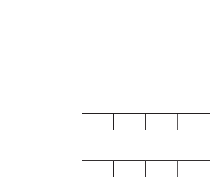
The nodal pressures and velocities are given in the table below.
Nozzle geometry and exact flow field using Bernoulli’s equation
Node A (m
2
) p (Pa) Node A (m
2
) u (m/s)
A 0.5 9.60000 1 0.45 0.99381
B 0.4 9.37500 2 0.35 1.27775
C 0.3 8.88889 3 0.25 1.78885
D 0.2 7.50000 4 0.15 2.98142
E 0.1 0
ANIN_C06.qxd 29/12/2006 09:59 AM Page 201
202 CHAPTER 6 ALGORITHMS FOR PRESSURE---VELOCITY COUPLING
The governing equations for steady, one-dimensional, incompressible, fric-
tionless equations through the planar nozzle are as follows:
Mass conservation: (
ρ
Au) = 0 (6.61)
Momentum conservation:
ρ
uA =−A (6.62)
These equations are familiar from introductory fluid mechanics texts. A
derivation has also been given in Appendix E.
Discretised u-momentum equation
The discretised form of momentum equation (6.62) is
(
ρ
uA)
e
u
e
− (
ρ
uA)
w
u
w
=∆V
where the right hand side represents the pressure gradient integrated over
the control volume ∆V and ∆p = p
w
− p
e
.
In standard notation the discretised momentum equation for this one-
dimensional problem can be written as
a
P
u*
P
= a
W
u*
W
+ a
E
u*
E
+ S
u
If we use the upwind differencing scheme the coefficients may be
obtained from (see Section 5.6)
a
W
= D
w
+ max(F
w
, 0)
a
E
= D
e
+ max(0, −F
e
)
a
P
= a
W
+ a
E
+ (F
e
− F
w
)
The flow is frictionless so there is no viscous diffusion term in the governing
equation, and hence D
w
= D
e
= 0. F
w
and F
e
are mass flow rates through the
west and east faces of the u-control volume. We compute the face velocities
needed for F
w
and F
e
from averages of velocity values at nodes straddling
the face and use the correct values of the west and east face area given in
the above table. At the start of the calculations we use the initial velocity
field generated from the guessed mass flow rate. For subsequent iterations
we use the corrected velocity obtained after solving the pressure correction
equation.
The source term S
u
contains the pressure gradient integrated over the
control volume:
S
u
=×∆V =×A
av
∆x =∆p × (A
w
+ A
e
)
Since the geometry has a varying cross-sectional area we use an averaged area
to calculate ∆V. At first glance this looks like a very crude approximation,
but it is possible to show that the accuracy order of S
u
is no worse than the
upstream differencing used for the momentum flux terms.
In summary the coefficients of the discretised u-equations are given by
F
w
=
ρ
A
w
u
w
and F
e
=
ρ
A
e
u
e
a
W
= F
w
a
E
= 0
1
2
∆p
∆x
∆p
∆x
∆p
∆x
dp
dx
du
dx
d
dx
Solution
ANIN_C06.qxd 29/12/2006 09:59 AM Page 202

6.10 WORKED EXAMPLES OF THE SIMPLE ALGORITHM 203
a
P
= a
W
+ a
E
+ (F
e
− F
w
)
S
u
=∆p ×
1
–
2
(A
w
+ A
e
) =∆p × A
P
The parameter d required in the pressure correction equations is calculated
at this stage from
d ==
Pressure correction equation
The discretised form of the continuity equation in this one-dimensional
geometry is
(
ρ
uA)
e
− (
ρ
uA)
w
= 0
The corresponding pressure correction equation is
a
P
p′
P
= a
W
p′
W
+ a
E
p′
E
+ b′
where a
W
= (
ρ
dA)
w
, a
E
= (
ρ
dA)
e
b′=(F *
w
− F *
e
)
Values of the parameter d come from discretised momentum equations (see
above and Section 6.4).
In the SIMPLE algorithm the pressure corrections p′ are used to compute
the velocity corrections u′ and the corrected pressure and velocity fields using
u′=d(p ′
I
− p′
I+1
)
p = p* + p′
u = u* + u′
Numerical values --- momentum equation
First we consider the internal nodes 2 and 3.
• Velocity node 2
F
w
= (
ρ
uA)
w
= 1.0 × [(u
1
+ u
2
)/2] × 0.4
= 1.0 × [(2.2222 + 2.8571)/2] × 0.4 = 1.01587
F
e
= (
ρ
uA)
e
= 1.0 × [(u
2
+ u
3
)/2] × 0.3
= 1.0 × [(2.8571 + 4.0)/2] × 0.3 = 1.02857
a
W
= F
w
= 1.01587
a
E
= 0
a
P
= a
W
+ a
E
+ (F
e
− F
w
) = 1.01587 + 0 + (1.02857 − 1.01587)
= 1.02857
S
u
=∆P × A
2
= (p
B
− p
C
) × A
2
= (7.5 − 5.0) × 0.35 = 0.875
The discretised momentum equation at node 2 is
1.02857u
2
= 1.01587u
1
+ 0.875
We also need to calculate the parameter d at this node for later use in
the pressure correction equation:
d
2
= A
2
/a
P
= 0.35/1.02857 = 0.34027
(A
w
+ A
e
)
2a
P
A
av
a
P
ANIN_C06.qxd 29/12/2006 09:59 AM Page 203

• Velocity node 3
We leave it as an exercise for the reader to check that application of the
above procedure at the control volume around node 3 yields
1.06666u
3
= 1.02857u
2
+ 0.625
and
d
3
= A
3
/a
P
= 0.25/1.06666 = 0.23437
Next we come to momentum control volumes 1 and 4, which need special
treatment because they both contain a boundary face.
• Velocity node 1
The stagnation pressure p
0
= 10 Pa is given in a plenum chamber
upstream from the inlet where the fluid is at rest. To carry out the
calculations we need conditions at the actual inlet plane of the
momentum control volume 1, which coincides with pressure node A.
At this location the velocity is non-zero and the actual pressure is lower
than the stagnation pressure due to acceleration of the flow as it enters
the nozzle. We denote the (as yet unknown) velocity at A by u
A
and use
Bernoulli’s equation to express the static pressure at A, which is needed
in the source term S
u
, in terms of p
0
and u
A
:
p
A
= p
0
− (
ρ
u
2
A
) (6.63)
Next we write u
A
in terms of the velocity u
1
using continuity:
u
A
= u
1
A
1
/A
A
(6.64)
Combining (6.63) and (6.64) yields
p
A
= p
0
−
ρ
u
2
1
2
(6.65)
Now we may write the discretised momentum equation for u-
momentum control volume 1 using the upwind scheme:
F
e
u
1
− F
w
u
A
= (p
A
− p
B
) × A
1
(6.66)
F
w
is calculated using the estimate u
A
from equation (6.64): i.e.
F
w
=
ρ
u
A
A
A
=
ρ
u
1
A
1
.
Substitution of expressions (6.64) and (6.65) into (6.66) gives
F
e
u
1
− F
w
u
1
A
1
/A
A
=[(p
0
−
1
–
2
ρ
u
2
1
(A
1
/A
A
)
2
) − p
B
] × A
1
(6.67)
Some rearrangement and placing all the terms involving pressures on
the right and those involving velocities on the left hand side yields
[F
e
− F
w
A
1
/A
A
+ F
w
×
1
–
2
(A
1
/A
A
)
2
]u
1
= (p
0
− p
B
)A
1
(6.68)
Hence, the central coefficient a
P
for this node is a
P
= F
e
− F
w
A
1
/A
A
+
F
w
×
1
–
2
(A
1
/A
A
)
2
. The first two contributions on the right hand side of
this formula come from the mass flux terms on the left hand side of
discretised momentum equation (6.66). The third term is an extra
contribution arising from our choice to specify the stagnation pressure at
inlet (this extra term would be omitted if a value of the static pressure
was specified at inlet instead).
D
E
F
A
1
A
A
A
B
C
1
2
1
2
204 CHAPTER 6 ALGORITHMS FOR PRESSURE---VELOCITY COUPLING
ANIN_C06.qxd 29/12/2006 09:59 AM Page 204

6.10 WORKED EXAMPLES OF THE SIMPLE ALGORITHM 205
Expression (6.68) can be used in that form, but in these calculations
we have chosen to place the negative contribution to coefficient a
1
on
the right hand side. Hence
[F
e
+ F
w
×
1
–
2
(A
1
/A
A
)
2
]u
1
= (p
0
− p
B
)A
1
+ F
w
A
1
/A
A
× u
old
1
(6.69)
where u
1
old
is the nodal velocity at the previous iteration
This is termed the deferred correction approach and can be effective in
stabilising the iterative process if the initial velocity field is based on a
very poor guess (see also Chapter 5 – QUICK and TVD).
Now we calculate
u
A
= u
1
A
1
/A
A
= 2.22222 × 0.45/0.5 = 2.0
F
w
= (
ρ
uA)
w
=
ρ
u
A
A
A
= 1.0 × 2.0 × 0.5 = 1.0
The exit mass flux F
e
is computed in the same way as for the internal
nodes:
F
e
= (
ρ
uA)
e
= 1.0 × [(u
1
+ u
2
)/2] × 0.4
= 1.0 × [(2.2222 + 2.8571)/2] × 0.4 = 1.01587
a
W
= 0
a
E
= 0
a
P
= F
e
+ F
w
×
1
–
2
(A
1
/A
A
)
2
= 1.01587 + 1.0 × 0.5 × (0.45/0.5)
2
= 1.42087
In the source term we apply p
0
= 10 Pa and the initial velocity
u
1
old
= 2.22222 m/s.
S
u
= (p
0
− p
B
)A
1
+ F
w
(A
1
/A
A
) × u
1
old
= (10 − 7.5) × 0.45 + 1.0 × (0.45/0.5) × 2.22222
= 3.125
The discretised momentum equation at node 1 is therefore
1.42087u
1
= 3.125
The parameter d at this node is
d
1
= A
1
/a
P
= 0.45/1.4209 = 0.31670
• Velocity node 4
F
w
= (
ρ
uA)
w
= 1.0 × [(u
3
+ u
4
)/2] × 0.2 = 1.06666
At the east boundary of momentum control volume 4 we have a fixed
pressure, but we do not have two velocities that straddle the east
boundary. To compute the mass flux across this boundary we impose
continuity:
F
e
= (
ρ
uA)
4
At the first iteration we can use the assumed mass flow rate, so we set
F
e
= 1.0 kg/s. Thus,
a
W
= F
w
= 1.06666
a
E
= 0
a
P
= a
W
+ a
E
+ (F
e
− F
w
) = 1.06666 + 0 + (1.0 − 1.06666) = 1.0
ANIN_C06.qxd 29/12/2006 09:59 AM Page 205
206 CHAPTER 6 ALGORITHMS FOR PRESSURE---VELOCITY COUPLING
In the momentum source term we apply the given exit boundary
pressure p
E
= 0 Pa:
S
u
=∆P × A
av
= (p
D
− p
E
) × A
4
= (2.5 − 0.0) × 0.15 = 0.375
The discretised momentum equation at node 4 is
1.0u
4
= 1.0666u
3
+ 0.375
The parameter d at this node is
d
4
= A
4
/a
P
= 0.15/1.0 = 0.15
To summarise, the u-momentum equations using upwind differencing are as
follows:
1.42087u
1
= 3.125
1.02857u
2
= 1.01587u
1
+ 0.875
1.06666u
3
= 1.02857u
2
+ 0.625
1.00000u
4
= 1.06666u
3
+ 0.375
These equations can be solved by forward substitution starting at node 1.
The solution is
u
1
m/s u
2
m/s u
3
m/s u
4
m/s
2.19935 3.02289 3.50087 4.10926
These are the guessed velocities used in the SIMPLE pressure correction
procedure. Therefore star (*) superscripts are used to refer to these u-values
in the pressure correction calculations below.
The d values are as follows:
d
1
d
2
d
3
d
4
0.31670 0.34027 0.23437 0.15000
Numerical values --- pressure correction equation
The internal nodes are B, C and D.
• Pressure node B
a
W
= (
ρ
dA)
1
= 1.0 × 0.3167 × 0.45 = 0.14251
a
E
= (
ρ
dA)
2
= 1.0 × 0.34027 × 0.35 = 0.11909
F *
w
= (
ρ
u*A)
1
= 1.0 × 2.199352 × 0.45 = 0.98971
F *
E
= (
ρ
u*A)
2
= 1.0 × 3.022894 × 0.35 = 1.05801
a
P
= a
W
+ a
E
= 0.14251 + 0.11909 = 0.26161
b′=F *
w
− F *
e
= 0.98971 − 1.05801 =−0.06830
The pressure correction equation at node B is
0.26161p ′
B
= 0.14251p ′
A
+ 0.11909p ′
C
− 0.06830
• Pressure nodes C and D
We leave it for the reader to check that the corresponding pressure
correction equations for nodes C and D are
ANIN_C06.qxd 29/12/2006 09:59 AM Page 206