Versteeg H., Malalasekra W. An Introduction to Computational Fluid Dynamics: The Finite Volume Method

Подождите немного. Документ загружается.

11.8 DISCRETISATION OF THE DIFFUSION TERM 317

Before developing an expression for the cross-diffusion term, we note that

the central difference on the right hand side of Equation (11.8) is of course

only actually an approximation of

∂φ

∂ξ

, whereas the left hand side actually

requires n . grad

∂φ

∂

n. If the mesh is orthogonal

∂φ

∂ξ

∂φ

∂

n and

the central difference approximation is correct, but if the mesh is non-

orthogonal

∂φ

∂ξ

may be very different from

∂φ

∂

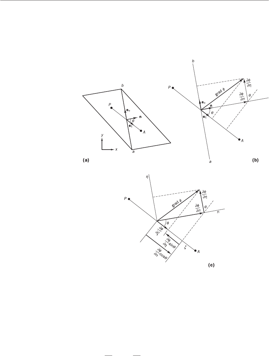
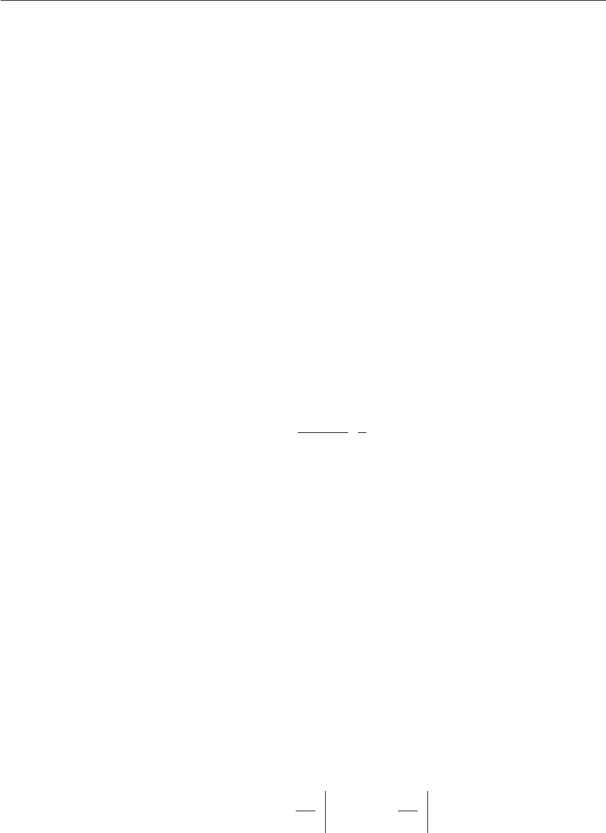
Figure 11.17 Deﬁnition sketch

for evaluation of cross-diffusion

term

Figures 11.17b–c show that

∂φ

∂ξ

corresponds to the length of the pro-

jection of vector grad

in the direction of

. Using the expression (11.9) we

can also represent grad

as the vector sum of the two components (

∂φ

∂

n)n

and (

∂φ

∂η

, as shown in Figure 11.17b. To get an improved estimate for

the normal ﬂux n . grad

∂φ

∂

n we examine the relationship between the

projection of grad

in the direction of

, i.e.

∂φ

∂ξ

, and the projections

in that direction of the two components (

∂φ

∂

n)n . e

and (

∂φ

∂η

. e

grad

. Figure 11.17 illustrates how the lengths of the projections of the

two component vectors can be calculated if the angle between the n- and

directions is denoted by

n . e

= cos(

) (11.13)

∂φ

∂

∂φ

∂

ANIN_C11.qxd 29/12/2006 04:43PM Page 317

and

. e

= − sin(

) (11.14)

The magnitude of the component of grad

in the direction of

is just

∂φ

∂ξ

which is also equal to the sum of the two projections (11.13) and (11.14).

Hence,

= cos(

) − sin(

) (11.15)

We remember that n . grad

∂φ

∂

n and rearrange (11.15) to obtain the

following expression for the normal component of the diffusive ﬂux required

in equation (11.8):

n . grad

== +tan(

) (11.16)

The two gradients of the transported quantity

on the right hand side of

expression (11.16) may both be approximated using central differencing:

= (11.17)

= (11.18)

where ∆

= d

is the distance between points A and P

and ∆

= d

is the distance between vertices a and b (=∆A

)

In the literature

∂φ

∂ξ

and

∂φ

∂η

are called the direct gradient and cross-

diffusion, respectively. Substitution of central difference approximations

(11.17) and (11.18) into equation (11.16) yields

n . grad

∆A

=+∆A

tan(

) (11.19)

It is straightforward to see in Figure 11.17 that

== (11.20)

and

tan(

) ==− (11.21)

Thus, (11.19) can be written in vector form as follows:

n . grad

∆A

=− (11.22)

Direct gradient term Cross-diffusion term

The factors n . n∆A

/n . e

and e

. e

∆A

/n . e

can be calculated from

the grid geometry. An alternative derivation to obtain equation (11.22) is

presented in Appendix F.

−

∆

. e

∆A

n . e

−

∆

n . n∆A

n . e

. e

n . e

sin(

)

cos(

)

n . n

n . e

cos(

)

−

∆

−

∆

∆A

cos(

)

−

∆

∂φ

∂η

−

∆

∂φ

∂ξ

∂φ

∂η

cos(

)

∂φ

∂ξ

∂φ

∂

∂φ

∂η

∂φ

∂

∂φ

∂ξ

∂φ

∂η

∂φ

∂η

318 CHAPTER 11 METHODS FOR DEALING WITH COMPLEX GEOMETRIES

ANIN_C11.qxd 29/12/2006 04:43PM Page 318

11.8 DISCRETISATION OF THE DIFFUSION TERM 319

Usually the cross-diffusion term is treated as a source term in the discret-

ised form. Therefore separating the cross-diffusion term equation (11.22) is

written as

n . grad

∆A

=+S

D-cross

(11.23)

To evaluate the cross-diffusion term the gradient of

along the line ab is

required. There are number of methods used for this calculation. One possibil-

ity is to interpolate nodal values of

to calculate

and

and use them to cal-

culate the gradient. Simple averaging over neighbouring nodes would lead to

= (11.24)

where N is the number of nodes surrounding the vertex a. Alternatively a

distance-weighted average may be used, which is more accurate but more

expensive to compute.

The gradient reconstruction methods described in the next section could

also be used to evaluate the gradient at vertices, and then linear interpolation

may be used to get the gradient at the face centre.

It can be seen that when the grid is orthogonal the unit vector e

and

the unit normal n are the same. Moreover, unit vectors e

and e

are per-

pendicular, so their dot product is zero and, hence, the cross-diffusion term

in equation (11.22) vanishes. Now, the ﬂux is given by equation (11.8).

In summary, for unstructured grids the diffusion ﬂux through each

control volume face is evaluated as follows:

n . Γ grad

∆A

= D

(

−

) + S

D-cross,i

(11.25)

where

= ∆A

and

D-cross,i

=−Γ

It should be noted that the diffusive ﬂux parameter D

has dimensions (kg/s)

of a mass ﬂow rate. This is different from the diffusion conductance D

(units kg/m

.s) that was used in Chapters 4 to 6, since D

includes the

control surface element area ∆A

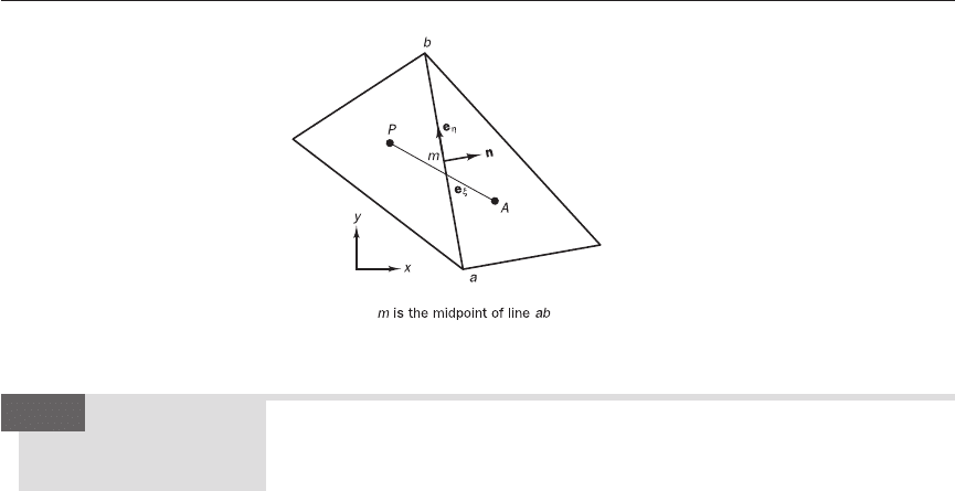
Figure 11.18 shows that there is a further error term due to the fact that

the central differences involved in the control surface element integration are

only second-order accurate if they are evaluated using the midpoint value of

n . grad

∆A

. This is not the case if the lines PA and ab do not intersect at

the midpoint m of ab when the grid is non-orthogonal. This error increases

with increasing skewness and aspect ratio, so it is important that every effort

is made to control skew and aspect ratios in unstructured grids.

−

∆

. e

∆A

n . e

n . n

n . e

∆

+ ...

−

∆

n . n∆A

n . e

ANIN_C11.qxd 29/12/2006 04:43PM Page 319

320 CHAPTER 11 METHODS FOR DEALING WITH COMPLEX GEOMETRIES

Figure 11.18 Geometric

sketch for skewed grid with

misalignment between midpoint

m of line ab and intersection

point of lines PA and ab

The convective term of equations (11.4) and (11.6) is

. (

ρφ

u)dA (11.26)

The area integral is evaluated as a sum of integrals over all control surface

elements ∆A

. Each of these integrals is approximated by the dot product

of the outward unit normal vector n

and a representative convective ﬂux

vector (

ρφ

u) multiplied by control surface element area ∆A

. We deﬁne con-

vective ﬂux parameter F

, which is equal to the mass ﬂow rate normal to the

surface element:

= n

. (

u)dA ≅ n

. (

u)∆A

(11.27)

Again we note that the units of the convective ﬂux parameter F

are those of

a mass ﬂow rate (kg/s), in contrast to the dimensions of the convective mass

ﬂux per unit area F used throughout Chapters 5 and 6, which has units

kg/m

.s.

The last step in equation (11.27) involves an approximation of the inte-

grand by means of a single representative velocity. A second-order accurate

calculation of F

using a single value is midpoint rule integration, which

requires the velocity vector u at the centre of the face i. In staggered grid

arrangements the face velocities are available from the momentum equation

and stored at face centres. On the other hand, in co-located grids it is neces-

sary to use interpolated face velocity components for the calculation of mass

ﬂux through the face. Special interpolation techniques are employed to over-

come the ‘checker-board’ pressure problem for a co-located arrangement.

We postpone discussion of these details until section 11.14.

On the assumption that we somehow have a suitable interpolated value

for the face velocity we can write the convective ﬂux of transported quantity

across the control surface in terms of the product as F

. (

ρφ

u)dA = F

(11.28)

where

is the value of

at the centre of surface area element i.

∑

all surfaces



∆A

∑

all surfaces



∆A



∆A

∑

all surfaces

Discretisation

of the convective

term

11.9

ANIN_C11.qxd 29/12/2006 04:43PM Page 320

11.9 DISCRETISATION OF THE CONVECTIVE TERM 321

As before, we also need to develop methods to generate face centre values

of the transported quantity which satisfy the requirements of conserva-

tiveness, boundedness and transportiveness that were formulated in Chapter

5. It should be noted that the treatment for general ﬂow variable

is also

applicable to velocity components u, v and w without change.

Upwind differencing scheme in unstructured grids

To calculate the convective ﬂux we may utilise the upwind approach, which

was introduced in section 5.6. The convective ﬂux is F

For F

> 0

For F

< 0

This is exact if the ﬂow vector u is also in the direction of PA (see Figure 11.15).

In a general situation the velocity vector may or may not be in the direction

of PA. We have also established in earlier discussions that when the ﬂow

vector is not in the direction of discretisation (i.e. PA) the upwind scheme

gives false diffusion. This strongly suggests that we should consider using

a higher-order scheme or a TVD scheme for the calculation of the convec-

tive ﬂux.

Higher-order differencing schemes in unstructured grids

Recall that in 1D Cartesian grids the linear upwind differencing scheme

given by equation (5.65) is

+∆x

where (

−

)/∆x is the gradient at P and ∆x/2 is distance from P to the

face e. The scheme uses an upwind-biased estimate of the gradient at P to

calculate the face value

. This can be extended formally to unstructured

meshes by using a Taylor series expansion of

about the centroid P:

(x, y) =

+ (∇

)

. ∆r + O (|∆r |

) (11.29)

where (∇

)

is the gradient of

at point P.

If we take ∆r as the distance vector from P to the face (see Figure 11.15)

then the face value of the transported quantity

can be evaluated by means

+ (∇

)

. ∆r (11.30)

Equation (11.29) indicates that the magnitude of the neglected terms is

proportional to the square of the distance between node P and the face i, so

this is a second-order approximation.

To use equation (11.30) in an unstructured grid to calculate

we need

∇

at the point P. In the literature there are several methods available to

calculate this quantity. One popular method is to use the so-called least-

squares gradient reconstruction at P.

Referring to Figure 11.19, the values of the transported quantity

at each

node surrounding the centre may be expressed as follows:

− x

) +

− y

) (11.31)

∂φ

∂

∂φ

∂

−

∆x

ANIN_C11.qxd 29/12/2006 04:43PM Page 321

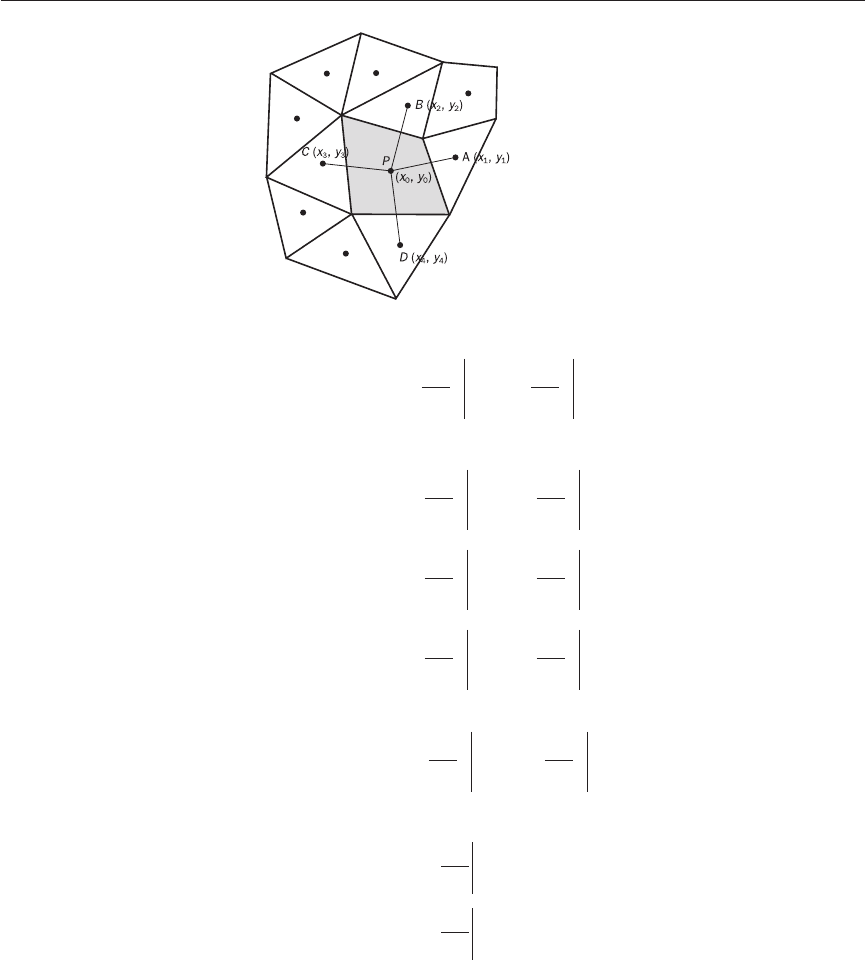
322 CHAPTER 11 METHODS FOR DEALING WITH COMPLEX GEOMETRIES

Figure 11.19 A control volume

and its neighbour nodes

Written in another form

∆x

∆y

(11.32)

For each node surrounding ‘0’ we have

−

∆x

∆y

(11.33a)

−

∆x

∆y

(11.33b)

−

∆x

∆y

(11.33c)



−

∆x

∆y

(11.33n)

This set of equations can be assembled into a matrix equation as follows:

G∆x

∆y

JG J G

−

H∆x

∆y

KH K H

−

H∆x

∆y

KH K = H

−

K (11.34)

HKH K H K

I∆x

∆y

LI L I

−

This represents an overdetermined system of linear equations, in the form

AX = B, which may be solved for X = [

∂φ

∂

∂φ

∂

] using the least-squares

approach. Multiplying both sides of the equation by transpose A

we obtain

AX = A

B (11.35)

Then A

A becomes a 2 × 2 matrix that can be easily inverted to solve for X.

Since matrix A depends on geometry only, this calculation needs to be done

once for each node. The required gradient vector is obtained from

X = (A

−1

B (11.36)

∂φ

∂

∂φ

∂

∂φ

∂

∂φ

∂

∂φ

∂

∂φ

∂

∂φ

∂

∂φ

∂

∂φ

∂

∂φ

∂

∂φ

∂

∂φ

∂

ANIN_C11.qxd 29/12/2006 04:43PM Page 322

11.9 DISCRETISATION OF THE CONVECTIVE TERM 323

Anderson and Bonhaus (1994) commented that this procedure can be very

inaccurate when the grid is highly stretched. For such applications these

authors recommended the QR decomposition method. Details of the QR

decomposition method can be found in Golub and Van Loan (1989). Further

details on gradient reconstruction can be found in Haselbacher and Blazek

(2000).

TVD schemes in unstructured grids

The concept of TVD schemes for the calculation of convective ﬂuxes was

introduced in Chapter 5. As explained there, higher-order schemes such as

QUICK can be accommodated in the TVD framework, which is the most

general form of discretisation scheme. Darwish and Moukalled (2003) have

provided a detailed discussion on the use of TVD schemes in unstructured

meshes. Here we summarise their development.

In the usual notation for Cartesian grids it was shown, in section 5.10, that

for the positive ﬂow direction, the face value of

using a TVD scheme may

be written as

+ (

−

) (11.37)

where r is the ratio of the upwind-side gradient to the downwind-side gradi-

ent given by

r = (11.38)

Here E is the downstream node and W is the upstream node. In relation to a

face of an unstructured cell A is equivalent to E .

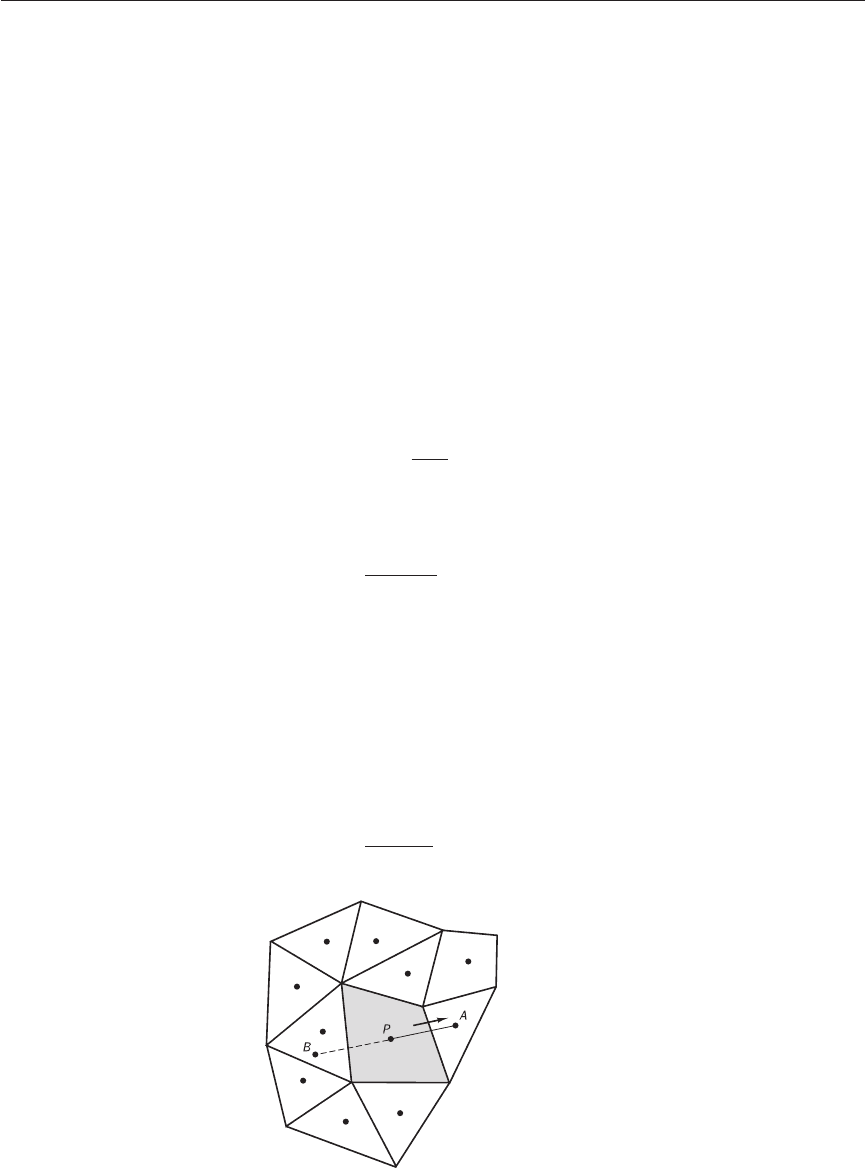
However, in unstructured grid arrangements the value of r cannot be

written in the same way because the upstream nodal value (assuming ﬂow

is positive along P to A) equivalent to W is not available. We need to con-

struct an upstream ‘dummy’ node B as shown in Figure 11.20 to be able to use

the standard approach. Details of such procedures can be found in Whitaker

et al. (1989) and Cabello et al. (1994). The value

at dummy node B might

be calculated by averaging over nearby nodal values. Thus, if

was available

r = (11.39)

−

(r)

Figure 11.20 Upwind dummy

node reconstruction for higher-

order schemes

ANIN_C11.qxd 29/12/2006 04:43PM Page 323

324 CHAPTER 11 METHODS FOR DEALING WITH COMPLEX GEOMETRIES

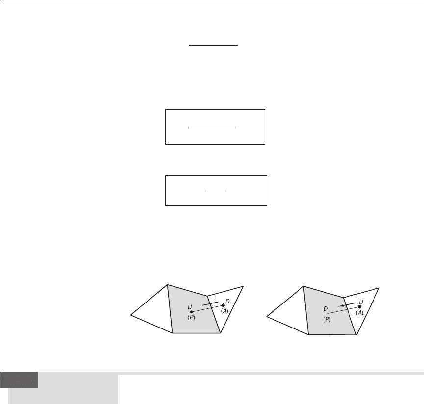
Figure 11.21 Selection of

upstream and downstream nodes

depending on ﬂow direction

Treatment of

source terms

Finally the source term in equation (11.4) is treated in the same way as we

did in Cartesian coordinates:

SdV = D∆V (11.43)

where ∆V is the volume of the control volume

D is the average of S over the control volume

A second-order accurate approximation of integral (11.43) is obtained

using the midpoint rule, which replaces the average D by the nodal value

of the source function S evaluated at the centroid of the control volume.

The source term is introduced to the discretised equation as before by using

D∆V = S

− S

. In 2D the volume is the area of the cell multiplied by

unit dimension in the direction normal to the 2D plane. In 3D ∆V is the vol-

ume of the control volume and can be calculated using standard geometrical

relationships and vector algebra. Kordula and Vinokur (1983), for example,

give a method to calculate volumes in an efﬁcient manner.



In the absence of

, Darwish and Moukalled (2003) recommend

r =−1 (11.40)

Here r

is the distance vector between nodes P and A. The ﬂow can be from

P to A or from A to P. To generalise the above expression we should adopt

the notation ‘U’ for upstream and ‘D’ for downstream:

r =−1 (11.41)

The TVD expression for convective ﬂux can also be written as

+ (

−

) (11.42)

where U denotes the upstream node and D denotes the downstream node.

Depending on the direction of the ﬂow vector along the line joining centroids

of the cells, the upstream and downstream points have to be selected appro-

priately and allocated to P and A: see Figure 11.21. The interested reader

should consult Darwish and Moukalled (2003) for further details.

(r)

(2∇

. r

)

−

(2∇

. r

)

−

11.10

ANIN_C11.qxd 29/12/2006 04:43PM Page 324

11.11 ASSEMBLY OF DISCRETISED EQUATIONS 325

The diffusion ﬂux through a face is

(

−

) + S

D-cross,i

(11.44)

Using a TVD scheme for convective ﬂux and treating the TVD contribution

as deferred correction as outlined in Chapter 5, the convective ﬂux through

a face is

[

(r)(

−

)/2] (11.45)

The source term for the volume is

+ S

(11.46)

When these are substituted into steady ﬂow equation (11.4)

n . (

ρφ

u)dA = n . (Γ grad

)dA + S

dV (11.47)

we obtain

[

(r)(

−

)/2] = [D

(

−

) + S

D-cross,i

]

+ (S

+ S

) (11.48)

In the above equation A stands for the centroid of each control volume

surrounding the point P. For the convective terms U and D have to be

appropriately allocated to P and A depending on the ﬂow direction across the

face. The use of vector algebra in the derivation of the relevant equations,

in conjunction with the deﬁnitions of the unit normal vectors and velocity

vectors, takes care of the ﬂow direction. We automatically recover the correct

magnitude and sign of F

The above equation can be rearranged as

=∑a

+ S

+∑S

D-cross,i

(11.49)

where a

=∑a

− S

+∑F

Here S

is a source term arising from deferred corrections from TVD or

higher-order schemes (see section 5.10). ∑S

D-cross,i

is the source term due to

cross-diffusion and ∑F

is the mass imbalance over all faces. Note that the

system of equations arising from the discretisation process is no longer a

banded matrix, since, depending on the shape of the control volume, the

nodes for transported quantity

may be connected to an arbitrary number

of neighbouring nodes in an unstructured mesh. Solution of the system

therefore requires techniques such as the multigrid method described in

Chapter 7 or the conjugate gradient method.

Application of the unstructured equations to Cartesian grids

We solve a source-free 1D convection–diffusion problem shown in Fig-

ure 11.22 using upwind differencing to demonstrate that we can recover

the Cartesian discretised equations presented in section 5.6 from equation

(11.48).

∑

all surfaces

∑

all surfaces



Assembly of

discretised

equations

11.11

ANIN_C11.qxd 29/12/2006 04:43PM Page 325

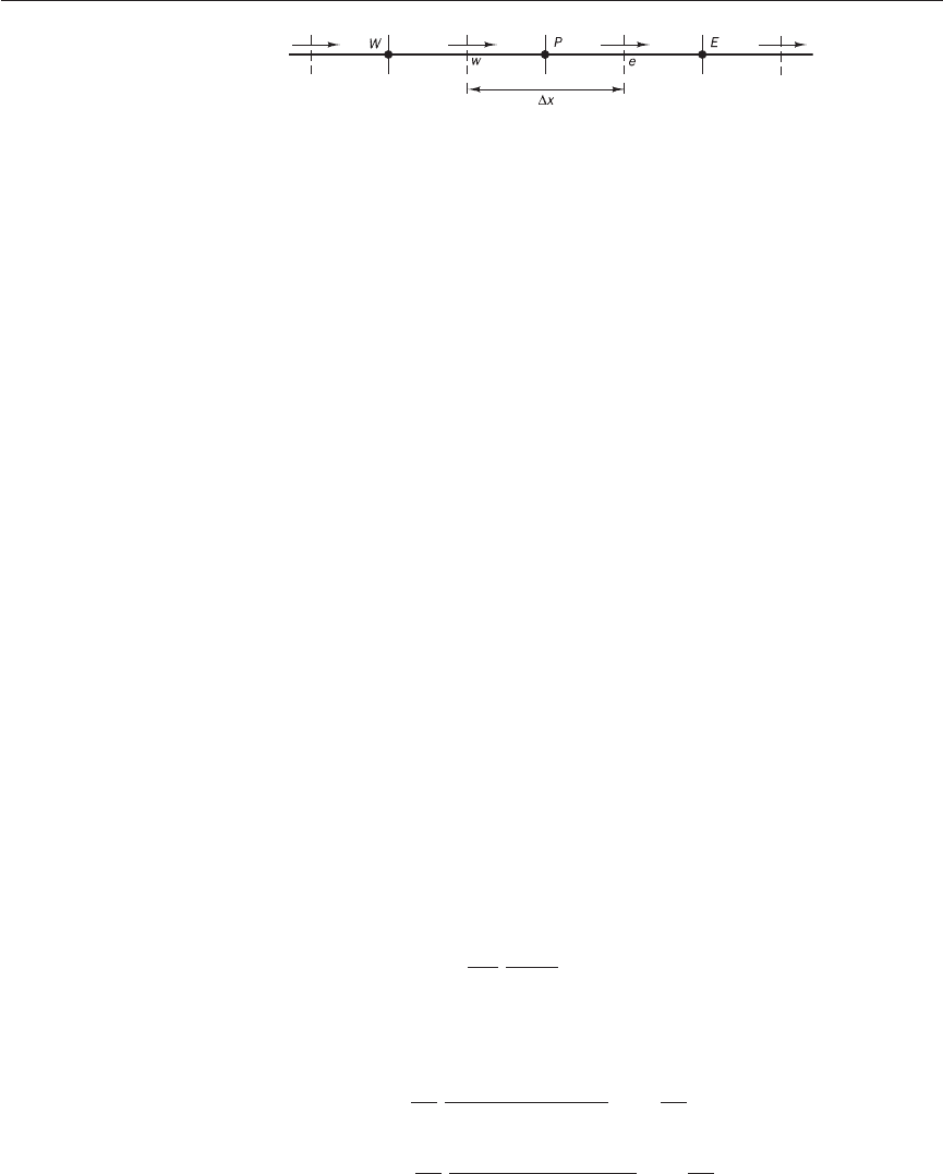
326 CHAPTER 11 METHODS FOR DEALING WITH COMPLEX GEOMETRIES

Figure 11.22 A 1D ﬂuid ﬂow

problem

The essential parameters used in equation (11.48) are control volume width

=∆x, the distance between nodes ∆

=∆x. For equally spaced control vol-

umes the distance between nodes is the same, i.e. ∆x

=∆x

=∆x. The

outward normal vector for the east face is

= 1i + 0j

The vector e

for the line PE is

= 1i + 0j

and the area of the east face is

∆A

= 1.0

The outward normal vector for the west face is

=−1i + 0j

The vector e

for the line PW is

=−1i + 0j

The area of the west face is

∆A

= 1.0

and the convection velocity vector is

u = ui + 0j

We use the standard notation for ﬂuid properties adopted in the previous

chapters: the diffusion coefﬁcient is denoted by Γ and the density by

Since the faces of the control volumes are perpendicular to the lines

joining nodes, no cross-diffusion terms arise in this orthogonal grid. Hence,

D-cross

= 0 and there is no source term. Thus, the diffusion ﬂux is given by

(11.22):

n . Γ grad

∆A

= D

(

−

)

where D

=∆A

Diffusion ﬂux parameters D

for the west and east faces from equation

(11.24) are

= 1.0 ==D

The mass ﬂow rate through the east face is

(1i + 0j) . (ui + 0j)1.0 =

u = F

∆x

(−1i + 1j) . (−1i + 1j)

∆x

(1i + 0j) . (1i + 0j)

∆x

n . n

n . e

∆x

ANIN_C11.qxd 29/12/2006 04:43PM Page 326