Versteeg H., Malalasekra W. An Introduction to Computational Fluid Dynamics: The Finite Volume Method
Подождите немного. Документ загружается.

11.3 CARTESIAN VS. CURVILINEAR GRIDS --- AN EXAMPLE 307
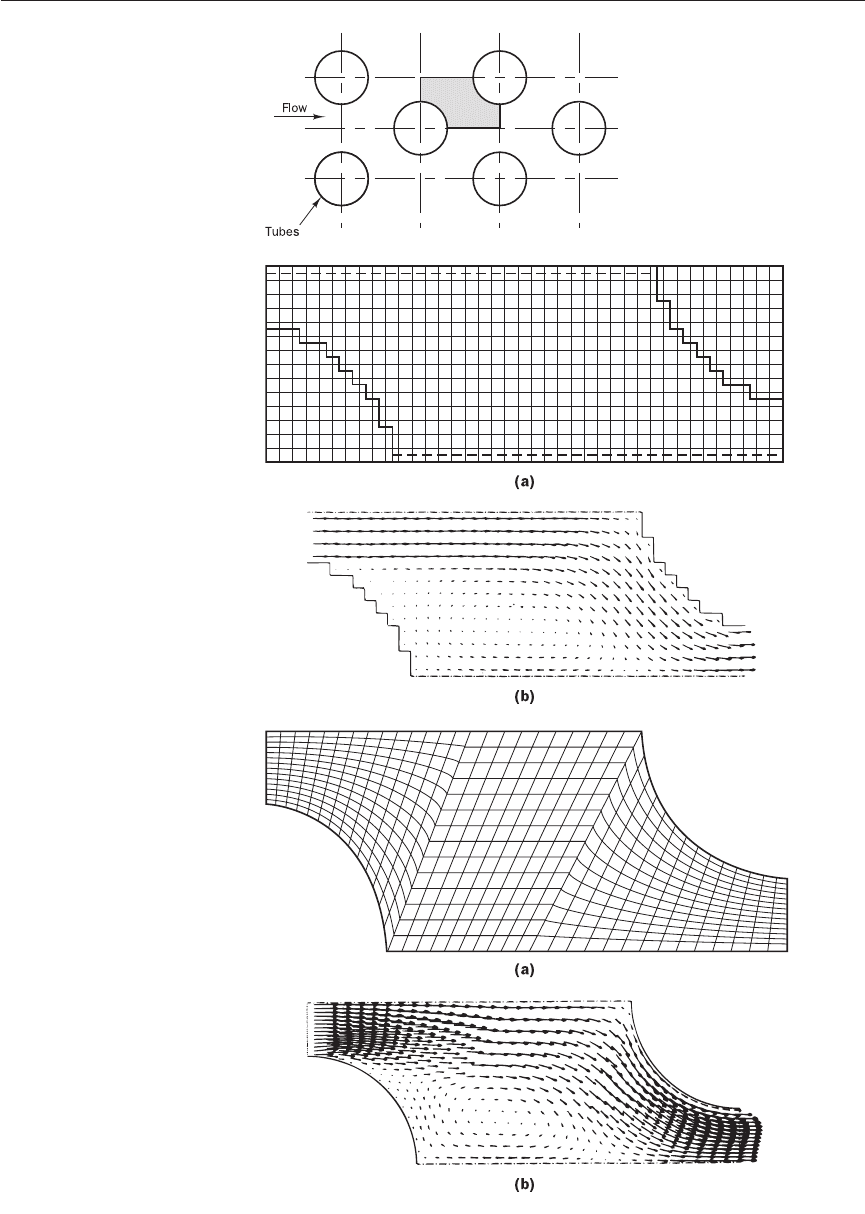
Figure 11.4 Flow over a heat
exchanger tube bank (only a part
shown)
Figure 11.5 (a) Cartesian grid
using an approximated profile
to represent cylindrical surfaces;
(b) predicted flow pattern using
a 40 × 15 Cartesian grid
Figure 11.6 (a) Non-orthogonal
body-fitted grid for the same
problem; (b) predicted flow
pattern using a 40 × 15
structured body-fitted grid
ANIN_C11.qxd 29/12/2006 04:43PM Page 307

Body-fitted grids have significant advantages over their Cartesian equiva-
lents, but there is a price to pay for the geometric flexibility: the governing
equations in curvilinear co-ordinate systems are much more complex. Detailed
discussions of the available methods of formulating the governing equations
can be found in Demirdzic (1982), Shyy and Vu (1991) and Ferziger and
Peric (2001). The main difference between the different formulations lies
in the grid arrangement and in the choice of dependent variables in the
momentum equations. In CFD procedures based on body-fitted co-ordinates
the use of non-staggered or co-located grid systems for velocities is increas-
ingly preferred to staggered grids, which require additional storage allocations.
However, special procedures are needed for non-staggered grids to ensure
proper velocity and pressure coupling and prevent the occurrence of checker-
board pressure oscillations identified in section 6.2. Unstructured grids also
use these co-located grid arrangements, and we discuss them further in
section 11.14.
In addition to the greater complexity of the equations, it should be noted
that body-fitted grids are still structured, so grid refinement is generally not
purely local. For example, in Figure 11.2 the refinement needed to resolve
the boundary layers and trailing edge geometry persists elsewhere in the
interior mesh. This shows up as regions of increased mesh density above,
below and downstream from the aerofoil roughly along three lines that
originate from the trailing edge. The number of mesh cells in the down-
stream direction is particularly large, which represents a waste of computer
storage.
Use of orthogonal and non-orthogonal body-fitted grids allows us to
capture the geometric details, but there can be difficulties associated with
their creation. To generate meshes that include all the geometrical details, it
is necessary to map the physical geometry into a computational geometry.
Mathematical details of the mapping process are not presented here; the
interested user should consult the relevant literature for details (see Thomson,
1984, 1988). An example of the mapping process for a part of a tube bank
is shown in Figures 11.7a–b. For this comparatively simple geometry it is
straightforward to develop a viable mapping, but when the domain geome-
try is more complex and/or involves a large number of internal objects this
can be a very tedious task.
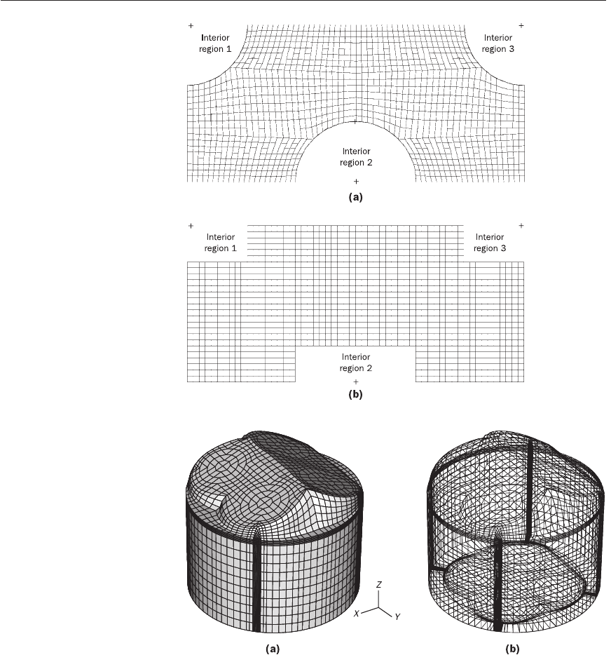
Figures 11.8a–b illustrate the difficulties of generating a body-fitted grid
for a pent-roof IC engine combustion chamber by mapping the cylinder
geometry into a single three-dimensional hexahedral block (Henson, 1998).
Valve details were created by carefully mapping the circular valves to square
regions. In addition, the grid had to accommodate piston bowl details, shown
on the surface mesh of Figure 11.8a. Various smoothing techniques were
used to improve the grid distributions, but the final grid still contains regions
with very acute angles and cells with undesirable aspect ratios, even after
smoothing. The four regions with dense surface mesh are the result of the
need to accommodate valve and pent-roof details. These groups of highly
skewed cells can lead to stability problems for CFD solvers. Such bad regions
in a mesh may have to be manually adjusted.
Therefore, in spite of their undoubted advantages over simple Cartesian
grids, the following problems are encountered with general orthogonal and
non-orthogonal structured grids:
308 CHAPTER 11 METHODS FOR DEALING WITH COMPLEX GEOMETRIES
Curvilinear
grids ---
difficulties
11.4
ANIN_C11.qxd 29/12/2006 04:43PM Page 308
11.4 CURVILINEAR GRIDS --- DIFFICULTIES 309
• Still difficult and time consuming to generate
• If the solution domain cannot be readily mapped into a rectangle (in 2D)
or rectangular parallelepiped (in 3D) this can result in skewed grid lines
causing unnecessary local variations
• Unnecessary grid resolutions can result in cases where mapping is
difficult
• Mapping is sometime impossible with complex 3D geometries with
internal objects/parts
Figure 11.7 Mapping
of physical geometry to
computational geometry in
structured meshes: (a) physical
grid in x, y co-ordinates; (b) the
mapped structure for (a) in the
computational domain
Figure 11.8 A structured
non-orthogonal mesh for a
pent-roof i.c. engine geometry
ANIN_C11.qxd 29/12/2006 04:43PM Page 309
To overcome the problems associated with structured grid generation for
complex geometries, block-structured CFD methods have been developed.
In a block-structured grid, the domain is sub-divided into regions, each
of which has a structured mesh. The mesh structure in each region can be
different, and it is even possible to use different co-ordinate systems. Such
meshes are more flexible than (‘single block’) structured meshes described
in the previous sections. The block-structured approach allows the use of
fine grids in regions where greater resolution is required. The interfaces
of adjacent blocks may have grids on either side that are matching or non-
matching, but, either way, they must be properly treated in a fully conserva-
tive manner. In some codes the solvers are applied in a block-wise manner
(block by block with overall final iterations to unify boundary conditions)
and local refinement is possible block-wise. Block-structured grids with
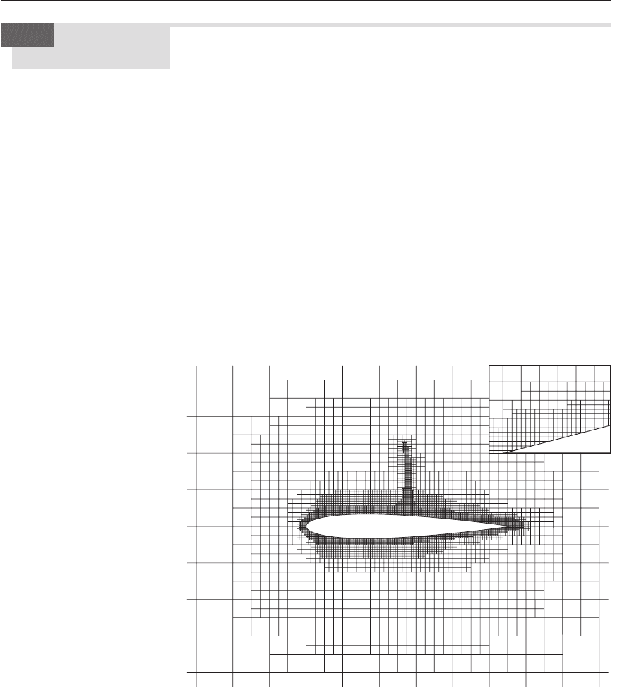
overlapping regions are called composite grids or chimera grids. Figure 11.9
shows a Cartesian block-structured grid used for the calculation of flow
over an aerofoil. The resulting grid structure combines the advantages of
Cartesian grids – easy to generate, equations simple to discretise and solve –
with the ability of curvilinear grids to accommodate curved complex bound-
aries (see Courier and Powell, 1996).
310 CHAPTER 11 METHODS FOR DEALING WITH COMPLEX GEOMETRIES
Figure 11.9 Block-structured
mesh for a transonic aerofoil.
Inset shows cut cells near aerofoil
surface. Also note additional grid
refinement in the flow region
to capture a shock above the
aerofoil
Source: Haselbacher (1999)
Block-structured
grids
11.5
Block-structured meshes are extremely useful in handling complex
geometries that consist of several geometrical sub-components such as the IC
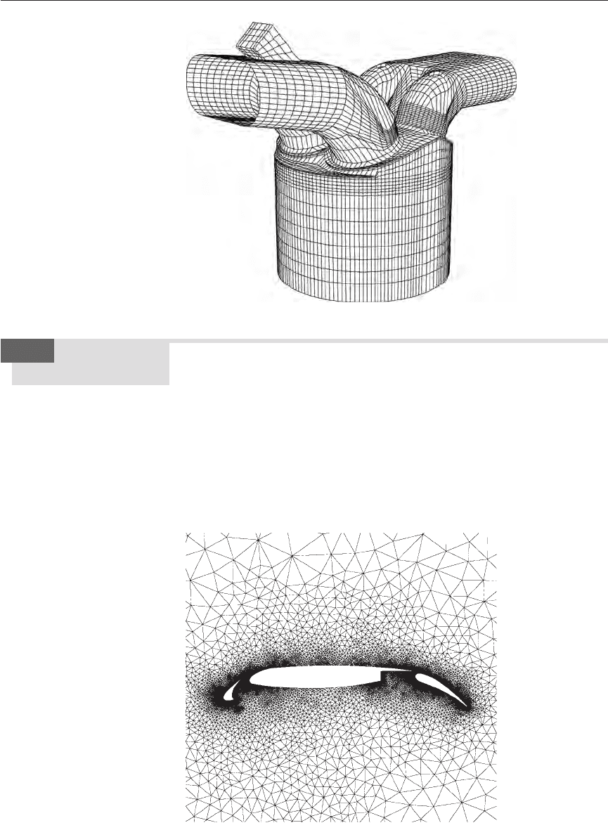
engine pent-roof cylinder and inlet port geometry. Figure 11.10 demon-
strates the improvement of grid quality that was achieved by applying the
block-structured meshing in the engine code KIVA-3V to define separate
blocks for mesh inlet ports, valve regions and the engine cylinder (generated
using the pre-processor of Kiva 3V: see Amsden, 1997).
ANIN_C11.qxd 29/12/2006 04:43PM Page 310
11.6 UNSTRUCTURED GRIDS 311
Figure 11.10 Block-structured
mesh arrangement for an engine
geometry, including inlet and
exhaust ports, used in engine
simulations with KIVA-3V
An unstructured grid can be thought of as a limiting case of a multi-block
grid where each individual cell is treated as a block. The advantage of such
an arrangement is that no implicit structure of co-ordinate lines is imposed
by the grid – hence the name unstructured – and the mesh can be easily
concentrated where necessary without wasting computer storage. Moreover,
control volumes may have any shape, and there are no restrictions on the
number of adjacent cells meeting at a point (2D) or along a line (3D). In prac-
tical CFD, triangles or quadrilaterals are most often used for 2D problems
and tetrahedral or hexahedral elements in 3D ones. Figure 11.11 shows a tri-
angular unstructured mesh for the calculation of a 2D flow over an aerofoil.
Unstructured
grids
11.6
Figure 11.11 A triangular grid
for a three-element aerofoil
Source: Haselbacher (1999)
ANIN_C11.qxd 29/12/2006 04:43PM Page 311
In unstructured grid arrangements we are not restricted to one particular
cell type, but it is possible to use a mixture of cell shapes. In 2D a mixture
of triangular and quadrilateral elements can be used to construct the grid. In
3D flow calculations combinations of tetrahedral and hexahedral elements
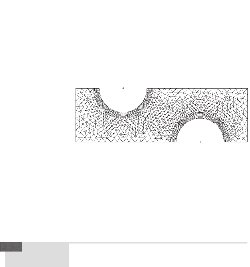
are frequently used. Such grids are called hybrid meshes. Figure 11.12
shows an example of a hybrid unstructured grid for the calculation of flow
in a tube bank where quadrilateral cells have been used near solid walls to
provide better resolution of the viscous effects in the boundary layers and
an expanding triangular mesh structure elsewhere to utilise the resources
efficiently.
312 CHAPTER 11 METHODS FOR DEALING WITH COMPLEX GEOMETRIES
Figure 11.12 An example of an
unstructured mesh with mixed
elements
Discretisation
in unstructured
grids
The most attractive feature of the unstructured mesh is that it allows
the calculation of flows in or around geometrical features of arbitrary
complexity without having to spend a long time on mesh generation and
mapping. Grid generation is fairly straightforward (especially with triangu-
lar and tetrahedral grids), and automatic generation techniques, originally
developed for finite element methods, are now widely available. Further-
more, mesh refinement and adaption (semi-automatic mesh refinement
to improve resolution in regions with large gradients) are much easier in
unstructured meshes. In the sections to follow we explore the unstructured
methodology in more detail as it is now the most popular technique and is
included in all commercial CFD codes on the market today.
Unstructured grids are the most general form of grid arrangement for
most complex geometries. Here we present a brief outline of discretisation
techniques for unstructured grids with arbitrary cell shapes, which may be
bounded by any number of control surfaces. We limit ourselves to the devel-
opment of the main ideas; interested readers should consult the literature for
further details of the methodology.
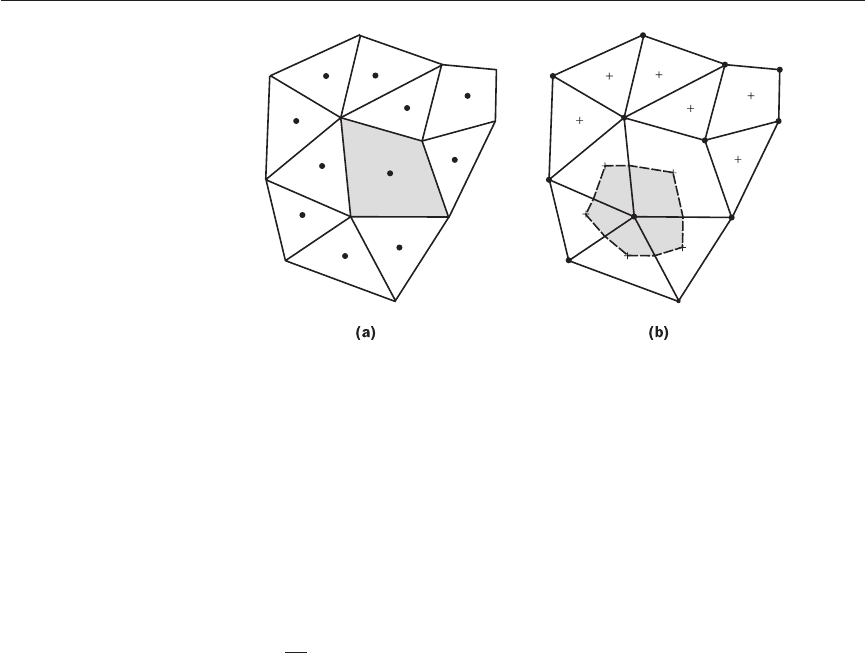
There are two ways of defining control volumes in unstructured meshes:
(i) cell-centred control volumes and (ii) vertex-centred control volumes.
These two variants are illustrated in Figure 11.13 for a 2D problem.
In the cell-centred method the nodes are placed at the centroid of the
control volume, as shown in Figure 11.13a. In the vertex-centred method
the nodes are placed on the vertices of the grid. This is followed by a process
known as median-dual tessellation, whereby sub-volumes are formed by
joining centroids of the elements and midpoints of the edges, as illustrated in
11.7
ANIN_C11.qxd 29/12/2006 04:43PM Page 312
11.7 DISCRETISATION IN UNSTRUCTURED GRIDS 313
Figure 11.13 Control volume
construction in 2D unstructured
meshes: (a) cell-centred control
volumes; (b) vertex-based control
volumes
Figure 11.13b. The sub-volume surrounding a node then forms the control
volume for discretisation. Both cell-centred and vertex-centred methods are
used in practice. We develop the ideas of discretisation in unstructured grids
for the cell-centred method, which is simpler to understand, and, since a
control volume always has more vertices than centroids, it has slightly lower
storage requirements than the vertex-centred method.
The discretisation in unstructured meshes can be developed from the
basic control volume technique introduced in earlier chapters, where we
used the integral form (2.40) of the conservation equation as the starting
point:
(
ρφ
)dV + div(
ρφ
u)dV = div(Γ grad
φ
)dV + S
φ
dV (11.1)
The volume integration in the transient term on the left hand side and
the source term on the right hand side can be conveniently evaluated as the
product of the volume of the cell and the relevant centroid value of the
integrand. The time integration can be treated using the explicit or implicit
techniques developed in Chapter 8.
Equation (11.1) also contains terms with the divergence of the convective
flux (
ρφ
u) and of the diffusive flux (Γ grad
φ
). In the absence of a specific
co-ordinate system these terms need careful treatment. We recall Gauss’s
theorem (2.41), which is applicable to any shape of control volume:
div a dV = n . a dA (11.2)
The surface integration must be carried out over the bounding surface A
of the control volume CV. The physical interpretation of n . a is the com-
ponent of the vector a in the direction of the outward unit vector n normal
to infinitesimal surface element dA.
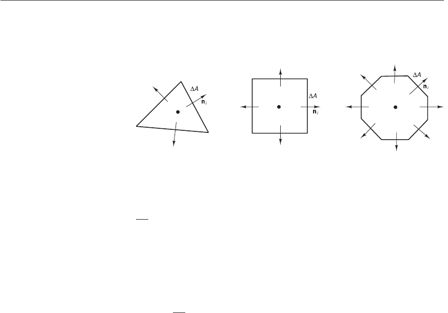
Some simple 2D examples of different shapes of control volumes are
shown in Figure 11.14. We note that the bounding surface or control surface
of each 2D control volume is a closed contour formed by means of a series of
finite-sized straight line elements, the area of which is denoted by ∆A. In 3D
A
CV
CV
CV
CV
∂
∂
t
CV
ANIN_C11.qxd 29/12/2006 04:43PM Page 313
314 CHAPTER 11 METHODS FOR DEALING WITH COMPLEX GEOMETRIES
Figure 11.14 Typical 2D
control volumes with varying
number of surface elements
the control volume would be bounded by triangular or quadrilateral surface
elements.
Application of Gauss’s theorem to equation (11.1) gives
ρφ
dV + n . (
ρφ
u)dA = n . (Γ grad
φ
)dA + S
φ
dV (11.3)
Note that A is the area of the entire control surface in equation (11.3) and dA
indicates an infinitesimal surface element. The area integrations are carried
out over all line segments (2D) or surface elements (3D), so they can be
written as follows:
ρφ
dV + n
i
. (
ρφ
u)dA
= n
i
. (Γ grad
φ
)dA + S
φ
dV (11.4)
For steady flows we have
n . (
ρφ
u)dA = n . (Γ grad
φ
)dA + S
φ
dV (11.5)
and hence
n
i
. (
ρφ
u)dA = n
i
. (Γ grad
φ
)dA + S
φ
dV (11.6)
To evaluate the control surface integrations we need expressions for flux
vectors (
ρφ
u) and (Γ grad
φ
) as well as geometric quantities n
i
and ∆A
i
. In
sections 11.7 and 11.8 we develop special expressions for the diffusive flux
n
i
. (Γ grad
φ
) and convective flux n
i
. (
ρφ
u) across line segments or surface
elements. Here we show how the outward normal vector n
i
and surface ele-
ment area ∆A
i
can be calculated using simple trigonometry and vector algebra
from the vertex co-ordinates of the unstructured grid.
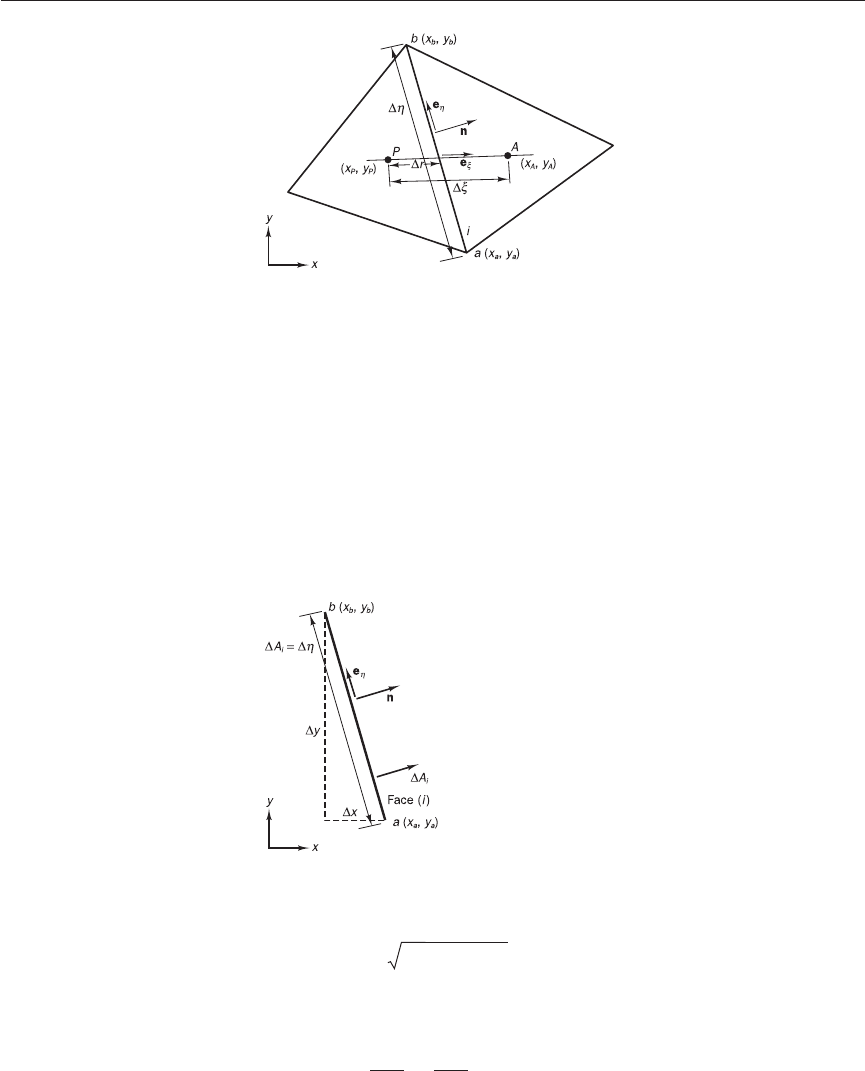
A typical cell-centred arrangement is shown in Figure 11.15 along with
the notations we will use to describe the discretisation procedure.
CV
∆A
i
∑
all surfaces
∆A
i
∑
all surfaces
CV
A
A
CV
∆A
i
∑
all surfaces
∆A
i
∑
all surfaces
D
E
F
CV
A
B
C
∂
∂
t
CV
A
A
D
E
F
CV
A
B
C
∂
∂
t
ANIN_C11.qxd 29/12/2006 04:43PM Page 314
11.7 DISCRETISATION IN UNSTRUCTURED GRIDS 315
Figure 11.15 Cell-centred
control volume arrangement
In this figure point P is the centroid of the control volume for which we
develop the discretisation process. Point A is the centroid of the adjacent
control volume and e
ξ
is a unit vector along the line joining P and A. The
face separating the two control volumes is identified as ‘i’, and ab is a line
joining vertices a and b, which are shared by the two control volumes. The
co-ordinates of points a and b are (x
a
, y
a
) and (x
b
, y
b
) respectively. Unit vectors
n and e
η
are, respectively, the outward normal vector and tangent vector to
face i.
We now calculate the required geometry parameters for equations (11.4)
and (11.6) as follows. Consider the control volume face shown in Figure 11.16.
Figure 11.16 A face of a control
volume and the normal unit
vector
The area of the face is given by
∆A
i
=
where ∆x = x
b
− x
a
and ∆y = y
b
− y
a
The normal unit vector to the surface is defined by
n = i − j (11.7)
In the absence of a grid structure it is necessary to create a data structure for
the geometry information along with a method of identifying the relationship
between vertices, cell indices, relevant edges and neighbouring cell indices.
∆x
∆
A
i
∆y
∆
A
i
(∆x)
2
+ (∆y)
2
ANIN_C11.qxd 29/12/2006 04:43PM Page 315

In equations (11.4) and (11.6) the diffusion term has been written as a sum
over all the surface elements that make up the bounding surface of a control
volume:
n
i
. (Γ grad
φ
)dA
The area integration for each of the elements is approximated by the dot
product of the outward unit normal vector n
i
and a representative diffusive
flux vector (Γ grad
φ
) for the control surface element ∆A
i
. The latter can be
approximated easily using the central differencing method along line PA.
Thus,
n
i
. (Γ grad
φ
)dA ≅ n
i
. (Γ grad
φ
)∆A
i
≅Γ ∆A
i
(11.8)
In equation (11.8) ∆
ξ
is the distance between the centroids A and P. It should
be noted that central difference (11.8) is only accurate if the line joining
nodes P and A and the unit normal vector n
i
are in the same direction, so the
approximation is only correct if the mesh is fully orthogonal. Generally, in
unstructured meshes the lines connecting centroids P and A are not parallel
to the unit normal vector n
i
, as shown in Figure 11.15. This is known as mesh
skewness or non-orthogonality. The flux calculation (11.8) therefore has to
be corrected by adding a contribution arising from non-orthogonality. There
are different ways to correct the flux (e.g. Davidson, 1996; Mathur and Murthy,
1997; Haselbacher, 1999; Kim and Choi, 2000; Ferziger and Peric, 2001),
but the most common form is to introduce a term known as cross-diffusion,
which is treated as a source term when the discretised equation is assembled.
We follow Mathur and Murthy (1997) and develop an expression for the
cross-diffusion term by introducing co-ordinates
ξ
along the line joining P
and A, and
η
along the face of the control volume (i.e. along the line joining
vertices a and b). Figure 11.17a shows that the outward unit normal vector
n
i
is perpendicular to the tangential co-ordinate
η
. Thus, the term grad
φ
can
be expressed in terms of x, y coordinates or n,
η
coordinates as follows:
grad
φ
= i + j = n + e
η
(11.9)
where n and e
η
are unit vectors along normal and tangential directions.
As an aside we note that the normal unit vector n and the two other unit
vectors e
ξ
and e
η
in the directions of
ξ
and
η
, respectively, can be calculated
from stored x- and y-co-ordinates of control volume nodes and vertices as
follows (see Figures 11.16 and 11.17a):
n = i − j = i − j (11.10)
e
ξ
= i + j (11.11)
e
η
= i + j (11.12)
y
b
− y
a
∆
η
x
b
− x
a
∆
η
y
A
− y
P
∆
ξ
x
A
− x
P
∆
ξ
x
b
− x
a
∆
η
y
b
− y
a
∆
η
∆x
∆
A
i
∆y
∆
A
i
∂φ
∂η
∂φ
∂
n
∂φ
∂
y
∂φ
∂
x
D
E
F
φ
A
−
φ
P
∆
ξ
A
B
C
∆A
i
∆A
i
∑
all surfaces
316 CHAPTER 11 METHODS FOR DEALING WITH COMPLEX GEOMETRIES
Discretisation of
the diffusion term
11.8
ANIN_C11.qxd 29/12/2006 04:43PM Page 316